Talking Tech: Applying LRMC Rankings to College Football, Part Two
The previous post in this series covered how LRMC works and its mathematical implementation. Now it's time to take things a step further and apply this concept to ranking college football teams.


This is the second and final part of a series on implementing LRMC rankings for CFB! This entry presupposes you are familiar with the mathematical concepts behind LRMC. To view part one, which covers these concepts, click here.
When we last left off, we covered how LRMC works and how to implement it mathematically. With our understanding of LRMC, we are now prepared to implement a version of LRMC computationally for ranking CFB teams. To start with, let's fire up our Python notebook.
import cfbd
import numpy as np
import pandas as pd
import matplotlib.pyplot as plt
from sklearn.linear_model import LinearRegression
import math
First, we'll grab a 6 year sample of CFB games, from 2015-2020 (you'll see why we're grabbing so many games in a second), then filter out any games not against BCS opponents.
seasons = [cfbd.GamesApi().get_games(year=iteryear, season_type='both') for iteryear in range(2015,2021)]
games = [game for season in seasons for game in season]

games_df = pd.DataFrame().from_records([
                dict(
                    id=g.id,
                    neutral_site=g.neutral_site,
                    home_team=g.home_team,
                    home_conference=g.home_conference,
                    home_points=g.home_points,
                    away_team=g.away_team,
                    away_conference=g.away_conference,
                    away_points=g.away_points,
                    season=g.season
                )
                for g in games
                if g.home_points is not None
                    and g.away_points is not None
                    and g.home_conference is not None
                    and g.away_conference is not None
            ])
games_df.head()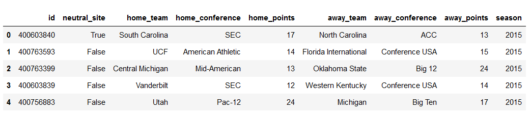
Our first task is to calculate rx for each of these games - the probability that the home team is better than the away team given their margin of victory.
For college basketball, estimating this value is quite easy with logistic regression – by virtue of conference home-and-home games, we can simply take all home-team margin of victories and run a logistic regression on the away game of the series to determine the odds of the home team winning on the road, then adjust for home court advantage. But since two teams playing each other twice in one season in college football are quite rare (let alone two teams playing a home-and-home series), we have to take a different approach. For college football, Kolbush and Sokol instead use a common-opponent approach for estimating rx[1]. Essentially, for a given game, we can look at the opponents Team A and Team B both played over the course of the season, and estimate the odds that Team A is better than Team B based on their win percentages against common opponents. Let's walk through an example.
games_df.loc[(games_df['id'] == 401112476)]
In this sample game, Miami lost to Virginia Tech by 7 points. How many opponents did Virginia Tech and Miami have in common that year?
opponents = games_df['away_team'][((games_df['home_team'] == 'Virginia Tech') & (games_df['season'] == 2019))].tolist() + games_df['home_team'][((games_df['away_team'] == 'Virginia Tech') & (games_df['season'] == 2019))].tolist() + games_df['away_team'][((games_df['home_team'] == 'Miami') & (games_df['season'] == 2019))].tolist() + games_df['home_team'][((games_df['away_team'] == 'Miami') & (games_df['season'] == 2019))].tolist()

common_opponents = set([team for team in opponents if opponents.count(team) > 1])

common_opponents
{'Duke', 'Georgia Tech', 'North Carolina', 'Pittsburgh', 'Virginia'}How well did VT and Miami do against those common opponents?
vt_w = 0
mia_w = 0
vt_g = 0
mia_g = 0
for index, game in games_df.loc[games_df['season'] == 2019].iterrows():
    if (game['home_team'] == 'Virginia Tech') & (game['away_team'] in common_opponents):
        vt_g += 1
        if game['home_points'] > game['away_points']:
            vt_w += 1
    elif (game['home_team'] == 'Miami') & (game['away_team'] in common_opponents):
        mia_g += 1
        if game['home_points'] > game['away_points']:
            mia_w += 1
    elif (game['away_team'] == 'Virginia Tech') & (game['home_team'] in common_opponents):
        vt_g += 1
        if game['away_points'] > game['home_points']:
            vt_w += 1
    elif (game['away_team'] == 'Miami') & (game['home_team'] in common_opponents):
        mia_g += 1
        if game['away_points'] > game['home_points']:
            mia_w += 1

print("Virginia Tech's common opponent WPCT: " + str(vt_w / vt_g))
print("Miami's common opponent WPCT: " + str(mia_w / mia_g))
Virginia Tech's common opponent WPCT: 0.6
Miami's common opponent WPCT: 0.4Virginia Tech won 60% of their games against their common opponents, and Miami won 40%. Per Kolbush and Sokol's approach, this renders our calculus rather simple. Let pj be the winning percentage of the home team (j) against common opponents between j and the away team (i), and pi be the winning percentage of i against common opponents, then rx becomes:
There is a 40% approximated chance Miami is better than Virginia Tech based on their common opponents.
To obtain a smooth estimate, we'll perform this for every game where teams had common opponents in a season, compile the point differentials for those games, then run a weighted logistic regression on those games (remember, our 40% estimate is currently independent of point differential – we wish to translate point differential into this estimate!). Our weights will be the total number of games played against common opponents for the teams in a given game[2].
We'll do this for the 2015-2018 seasons to estimate coefficients for the 2019 season (Kolbush and Sokol also used four prior seasons of data to estimate coefficients for a given season[1]). We'll also filter out neutral site games so we can get a better approximation for home field advantage.
train_games_df = games_df.loc[(games_df['season'].isin([2015,2016,2017,2018])) & (~games_df['neutral_site'])]

train_df = []

for index, game in train_games_df.iterrows():
    season = game['season']
    team_a = game['home_team']
    team_b = game['away_team']
    home_diff = game['home_points'] - game['away_points']
    opponents = train_games_df['away_team'][((games_df['home_team'] == team_a) & (games_df['season'] == season))].tolist() + games_df['home_team'][((games_df['away_team'] == team_a) & (games_df['season'] == season))].tolist() + games_df['away_team'][((games_df['home_team'] == team_b) & (games_df['season'] == season))].tolist() + games_df['home_team'][((games_df['away_team'] == team_b) & (games_df['season'] == season))].tolist()
    common_opponents = set([team for team in opponents if opponents.count(team) > 1])
    if len(common_opponents) > 1:
        a_w = 0
        b_w = 0
        a_g = 0
        b_g = 0
        for index, game in games_df.loc[(games_df['season'] == season) &
                                        ((games_df['home_team'].isin([team_a,team_b])) |
                                          games_df['away_team'].isin([team_a,team_b]))].iterrows():
            if (game['home_team'] == team_a) & (game['away_team'] in common_opponents):
                a_g += 1
                if game['home_points'] > game['away_points']:
                    a_w += 1
            elif (game['home_team'] == team_b) & (game['away_team'] in common_opponents):
                b_g += 1
                if game['home_points'] > game['away_points']:
                    b_w += 1
            elif (game['away_team'] == team_a) & (game['home_team'] in common_opponents):
                a_g += 1
                if game['away_points'] > game['home_points']:
                    a_w += 1
            elif (game['away_team'] == team_b) & (game['home_team'] in common_opponents):
                b_g += 1
                if game['away_points'] > game['home_points']:
                    b_w += 1

        r_x = ((a_w / a_g) + (1 - (b_w / b_g))) / 2

        d = {
            'season' : season,
            'team_a' : team_a,
            'team_b' : team_b,
            'home_diff' : home_diff,
            'r_x' : r_x,
            'weight' : a_g+b_g
        }
        train_df.append(d)

train_df = pd.DataFrame(train_df)
train_df.head()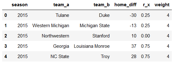
Now, we'll use our data to make a logistic regression model. Okay, I lied, it's not a strict logistic regression model – because we have a series of continuous probabilities to train on rather than a series of 1s and 0s (which a logistic regression model is usually trained upon), we're going to use the logit transformation to linearize our data, then run a weighted linear regression model, then undo the logit transformation to obtain probabilities for rx. Before we do that, we're going transform any probabilities of 100% to 90% and 0% to 10% – the logit transformation can't handle these specific probabilities, and speaking realistically, it would be difficult to project anyone as having a 100% chance of beating a given opponent regardless of their margins of victory against other opponents[3].
train_df.loc[train_df['r_x'] == 1,'r_x'] = 0.9
train_df.loc[train_df['r_x'] == 0,'r_x'] = 0.1
x = np.array(train_df['home_diff']).reshape(-1,1)
y = np.log(train_df['r_x'] / (1 - train_df['r_x']))
w = train_df['weight']
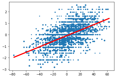
model = LinearRegression().fit(x, y, w)
plt.scatter(x, y, s = w)
plt.plot(x, model.predict(x), color='red', linewidth=3, label='Weighted model')
a = model.coef_[0]
b = model.intercept_
print("a = " + str(a))
print("b = " + str(b))a = 0.023983237378834784
b = -0.09541138612221126
Remember that for a linear regression, we find our coefficients in the form y = ax + b. Since y is logit transformed, to undo that transformation, we plug ax + b into e(y) / (1 + e(y)) to get e(ax + b) / (1 + e(ax + b)).
Let's return to that Virginia Tech/Miami game. Based on the point differential of the game and our model, what are the odds that Miami was better than Virginia Tech?
print(math.exp(a * -7 + b) / (1 + math.exp(a * -7 + b)))0.43455413139478277
Not too far off from our original estimate of 40%!
We can also quickly calculate the expected home field advantage from these coefficients[4]:
h = (-b / a)
print(h)
3.9782530029249448
So from 2015-2018, home field advantage appears to be worth about 4 points – not too far off from the 2.5 estimate Bill has been using in his SRS calculations.
Now that we have our formula for estimating rx, we can start building our Markov chain. Recall how we did this by hand in part one:
To generate our transition matrix, we sum up for games involving a particular team (let's say, Team X) by team. In the row of Team X, we place each team's sum of rx in each team's corresponding column (including Team X). Then, we divide all of the values in the row by the number of games Team X played.
We're going to implement this algorithmically for our 2019 dataset. First, let's grab our 2019 values.
games_df_2019 = games_df.loc[games_df['season'] == 2019]
games_df_2019.head()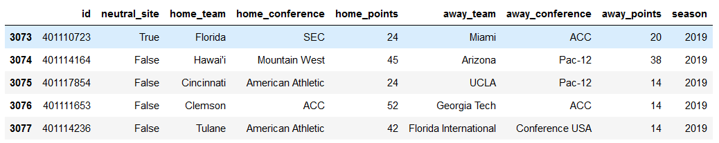
Next, we'll build two matrices: an n x n transition matrix, where n is the number of BCS teams, and a 1 x n matrix, tracking how many games each team plays.
team_names = sorted(list(set(games_df_2019['home_team'].tolist() + games_df_2019['away_team'].tolist())))
n_teams = len(team_names)
p = np.zeros((n_teams,n_teams))
n_games = np.zeros(n_teams)
Now, we'll iterate through each game, calculate rx, and put either rx or 1 - rx in the appropriate place in our transition matrix (to understand why we're playing each value where we are, consult part one of this guide here). For neutral-site games, we'll calculate rx after adding the home-field advantage in. We'll also add a game to each team's n_games counter.
for index, game in games_df_2019.iterrows():
    home_team = game['home_team']
    away_team = game['away_team']
    home_points = game['home_points']
    away_points = game['away_points']
    neutral_flg = game['neutral_site']
    home_team_ndx = team_names.index(home_team)
    away_team_ndx = team_names.index(away_team)
    spread = home_points - away_points
    if neutral_flg:
        spread += h
    r_x = math.exp(a * spread + b) / (1 + math.exp(a * spread + b))
    n_games[home_team_ndx] += 1
    n_games[away_team_ndx] += 1
    p[home_team_ndx, away_team_ndx] += 1 - r_x
    p[away_team_ndx, home_team_ndx] += r_x
    p[home_team_ndx, home_team_ndx] += r_x
    p[away_team_ndx, away_team_ndx] += 1 - r_x
Next, we'll divide each row of our transition by the number of games we're tracking for each team.
p = p / n_games[:,None]
print(p)
Finally, we'll approximate the steady state of this matrix to find what team LRMC believes is the best, then multiply our steady state matrix by a vector that counts down from n_teams to 1, which gives us our relative team strength.
prior = n_teams - np.array(list(range(n_teams)))
steady_state = np.linalg.matrix_power(p, 1000)
rating = prior.dot(steady_state)
rating_df = pd.DataFrame({
    'team': team_names,
    'lrmc_rating': rating

})
print(rating_df.sort_values(by=['lrmc_rating'], ascending=False).iloc[0:25])
team lrmc_rating
77 Ohio State 187.106455
48 LSU 175.945528
21 Clemson 157.969142
128 Wisconsin 130.052698
2 Alabama 129.821806
34 Georgia 118.031678
82 Oregon 115.817995
78 Oklahoma 110.981205
9 Auburn 108.585276
75 Notre Dame 107.732058
59 Michigan 106.242719
117 Utah 105.915359
84 Penn State 105.042793
12 Baylor 103.884959
101 Texas 101.253766
42 Iowa 100.165017
29 Florida 96.009519
56 Memphis 93.568406
62 Minnesota 90.033058
20 Cincinnati 89.598700
123 Washington 88.540195
43 Iowa State 88.377904
3 Appalachian State 86.243448
110 UCF 86.078021
102 Texas A&M 84.039906
These are some good looking rankings! Most importantly, it seems to be placing G6 teams in the sweet spot of where they usually end up year-to-year (10-3 UCF was also ranked 24th in the AP poll in 2019), which indicates that it's appropriately evaluating strength of schedule.
So we've finished with LRMC rankings with 2019 – but how will they work in the messed-up year of 2020, when some teams are playing conference-only schedules? Let's find out. We'll re-run the same analysis but we'll adjust home field advantage for the weird-pandemic stuff, eyeballing it and dropping it by 2 points – removing some to account for the impact of reduced or no crowd, but keeping some to account for rest/travel.
train_games_df = games_df.loc[(games_df['season'].isin([2016,2017,2018,2019])) & (~games_df['neutral_site'])]

train_df = []

for index, game in train_games_df.iterrows():
    season = game['season']
    team_a = game['home_team']
    team_b = game['away_team']
    home_diff = game['home_points'] - game['away_points']
    opponents = train_games_df['away_team'][((games_df['home_team'] == team_a) & (games_df['season'] == season))].tolist() + games_df['home_team'][((games_df['away_team'] == team_a) & (games_df['season'] == season))].tolist() + games_df['away_team'][((games_df['home_team'] == team_b) & (games_df['season'] == season))].tolist() + games_df['home_team'][((games_df['away_team'] == team_b) & (games_df['season'] == season))].tolist()
    common_opponents = set([team for team in opponents if opponents.count(team) > 1])
    if len(common_opponents) > 1:
        a_w = 0
        b_w = 0
        a_g = 0
        b_g = 0
        for index, game in games_df.loc[(games_df['season'] == season) &
                                        ((games_df['home_team'].isin([team_a,team_b])) |
                                          games_df['away_team'].isin([team_a,team_b]))].iterrows():
            if (game['home_team'] == team_a) & (game['away_team'] in common_opponents):
                a_g += 1
                if game['home_points'] > game['away_points']:
                    a_w += 1
            elif (game['home_team'] == team_b) & (game['away_team'] in common_opponents):
                b_g += 1
                if game['home_points'] > game['away_points']:
                    b_w += 1
            elif (game['away_team'] == team_a) & (game['home_team'] in common_opponents):
                a_g += 1
                if game['away_points'] > game['home_points']:
                    a_w += 1
            elif (game['away_team'] == team_b) & (game['home_team'] in common_opponents):
                b_g += 1
                if game['away_points'] > game['home_points']:
                    b_w += 1

        r_x = ((a_w / a_g) + (1 - (b_w / b_g))) / 2

        d = {
            'season' : season,
            'team_a' : team_a,
            'team_b' : team_b,
            'home_diff' : home_diff,
            'r_x' : r_x,
            'weight' : a_g+b_g
        }
        train_df.append(d)

train_df = pd.DataFrame(train_df)
train_df.loc[train_df['r_x'] == 1,'r_x'] = 0.9
train_df.loc[train_df['r_x'] == 0,'r_x'] = 0.1

x = np.array(train_df['home_diff']).reshape(-1,1)
y = np.log(train_df['r_x'] / (1 - train_df['r_x']))
w = train_df['weight']
model = LinearRegression().fit(x, y, w)
a = model.coef_[0]
b = model.intercept_
h = (-b / a) - 2

games_df_2020 = games_df.loc[games_df['season'] == 2020]
games_df_2020.head()

team_names = sorted(list(set(games_df_2020['home_team'].tolist() + games_df_2020['away_team'].tolist())))
n_teams = len(team_names)
p = np.zeros((n_teams,n_teams))
n_games = np.zeros(n_teams)

for index, game in games_df_2020.iterrows():
    home_team = game['home_team']
    away_team = game['away_team']
    home_points = game['home_points']
    away_points = game['away_points']
    neutral_flg = game['neutral_site']
    home_team_ndx = team_names.index(home_team)
    away_team_ndx = team_names.index(away_team)
    spread = home_points - away_points
    if neutral_flg:
        spread += h
    r_x = math.exp(a * spread + b) / (1 + math.exp(a * spread + b))
    n_games[home_team_ndx] += 1
    n_games[away_team_ndx] += 1
    p[home_team_ndx, away_team_ndx] += 1 - r_x
    p[away_team_ndx, home_team_ndx] += r_x
    p[home_team_ndx, home_team_ndx] += r_x
    p[away_team_ndx, away_team_ndx] += 1 - r_x

p = p / n_games[:,None]
prior = n_teams - np.array(list(range(n_teams)))
steady_state = np.linalg.matrix_power(p, 1000)
rating = prior.dot(steady_state)
rating_df = pd.DataFrame({
    'team': team_names,
    'lrmc_rating': rating

})
print(rating_df.sort_values(by=['lrmc_rating'], ascending=False).iloc[0:25])
team lrmc_rating
2 Alabama 135.230015
16 Buffalo 131.356858
21 Clemson 130.404969
73 Notre Dame 129.633899
10 BYU 129.319638
22 Coastal Carolina 113.635301
42 Iowa State 110.743776
49 Louisiana 109.852425
107 UCF 105.703515
20 Cincinnati 104.514956
69 North Carolina 103.885852
124 Western Michigan 103.099373
76 Oklahoma 100.090273
104 Tulane 99.269570
18 Central Michigan 99.083950
28 Florida 98.579495
14 Boston College 97.503712
56 Miami 96.908824
102 Toledo 96.386918
64 NC State 95.923478
52 Louisville 94.467302
98 Texas 93.446952
3 Appalachian State 93.341825
118 Virginia Tech 92.720235
33 Georgia 92.415851
These ratings are obviously a little rough, for various reasons – Buffalo has played just 4 games and thoroughly dominated their MAC-only opponents in three of them, and since our LRMC model doesn't account for sample size, they appear to be far better than they likely are – but I think it is worth pointing out that the rest of the rankings are more than plausible, and what's more, this ratings system actually resolves instead of base SRS.
Further, this method is largely empirical – the only manual adjustment we've made is to our estimate of home field advantage; the rest of it has required no manual adjustments. Bill's conference-adjusted SRS values are likely closest to what the top 25 ratings will look like, but this method is more robust in that it works with relatively few manual adjustments from year-to-year given the oddity of the 2020 season. I think there are advantages and disadvantages to either approach, and you should weigh those before applying the rating technique of your choosing. Still, LRMC, in both normal times and odd, is a powerful, useful tool for estimating team strength, and worthy of consideration for use in rankings.
To view the notebook for this code, click here.
[2] If j has a common opponent winning percentage of 100% and i has a common opponent winning percentage of 0%, that difference is far less meaningful if j and i have just one game against a common opponent, and far more meaningful if j and i have 10+ combined games against common opponents. Weighing our regression reflects the amount of confidence we have in our estimate of rx relative to other samples.
[3] You might have noticed that we make no adjustments here for running up the score, as most SRS implementations do. Why is that? Due to the sigmoid curve of a logistic regression function, running up the score yields diminishing returns as far as LRMC's ratings go.
[4] This is a little different from our calculation of home field advantage from part one – in part one, we used home point differential to estimate road winning percentage for a given matchup (sx), then adjusted for home field advantage to find rx. But here, we fit home point differential on a location-neutral estimate of team strength, so there isn't an intermediate sx to deal with. In math terms, when sx = 50%, x / 2 = h, when rx = 50%, x = h. We use both of these steps in part one, but here we only need the second step.