Talking Tech: Building an Artifical Neural Network to Predict Games

In this edition of Talking Tech, we're going to be diving into some machine learning. Specifically, we're going to be looking at my preferred method for building predictive models for just about anything: the artificial neural networks, or ANN for short. The name may sound intimidating, but ANNs aren't really any more difficult to build than other types of models.
So why do I like ANNs so much? They are fantastic for solving just about any type of complex problem. They are often used in anything from image classification to natural language processing. And while they are built on some very fancy math, they don't really require you to dive too deep into the math because there are some great libraries that abstract over those details. Now, there are different types and flavors of ANN architectures that may indeed require you to dig into the math more, but for simple ANNs like we will be building, there's no need to get into all of that. And that's the beauty of them, they can be quite simple to implement but there are also more complex implementations for more complex problems.
The main major drawback to ANNs, which holds true for just about any kind of machine learning algorithm, is that the resulting model is largely a black box. What do I mean by that? If someone were to ask you how much your model factors X feature or Y feature into making its predictions, you're not going to be able to tell them. You can tell them the features that are input into your model, but you won't really be able to tell them how those inputs are weighted. Yes, it will be possible to look up the weights in your trained model, but not in a way that's useful for these types of conversations.
Neural Networks, Explained
Artificial neural networks, otherwise just called neural networks, have a history that goes all the way back to the 1940s. As the name might suggest, they actually are inspired by biology and were initially meant to model real-life neural networks like those found in the brain. As such, you'll see all sorts of biology terminology used when describing artificial neural networks.
Before we get going, I should note that artificial neural networks are not as intimidating as they may seem. As we dive into how neural networks are built, it might seem like a lot of work but there are some great libraries that abstract over a lot of these details and make building these things super simple. However, I always think it's important to have an understanding of what's going on under the covers. So if you start getting intimidated as we go through this section, stick with it until we get to the actual coding part of this post as that part of this isn't too crazy and it will be worthwhile.
Artificial neural networks are built using a collection of interconnected nodes called neurons, again meant to represent the neurons in the brain. Every neuron in the network takes in inputs and produces an output, which can then be fed to several more connected neurons as part of their own input. These nodes are typically grouped into layers of neurons, of which there are three types:
- Input layer - There is typically one layer of input nodes where initial feature data is fed and output produced.
- Hidden layers - There can be several hidden layers of neurons, but there is always at least one of these. These layers receive output from either the input layer or another hidden layer as their own input and then produce their own output.
- Output layer - There is always one output layer that receives the output from the last hidden layer in the network as its own input and then produces the final output of the network.
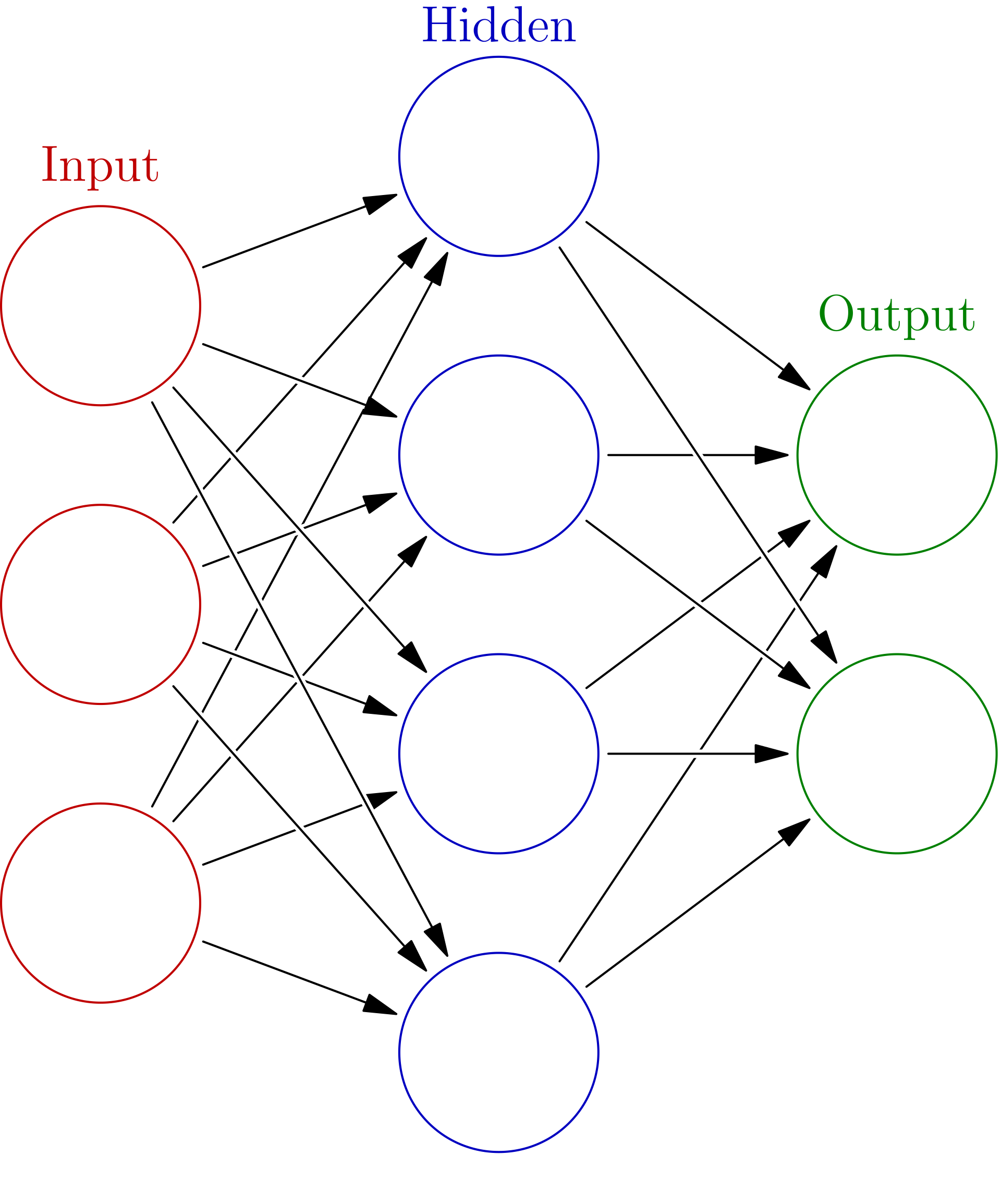
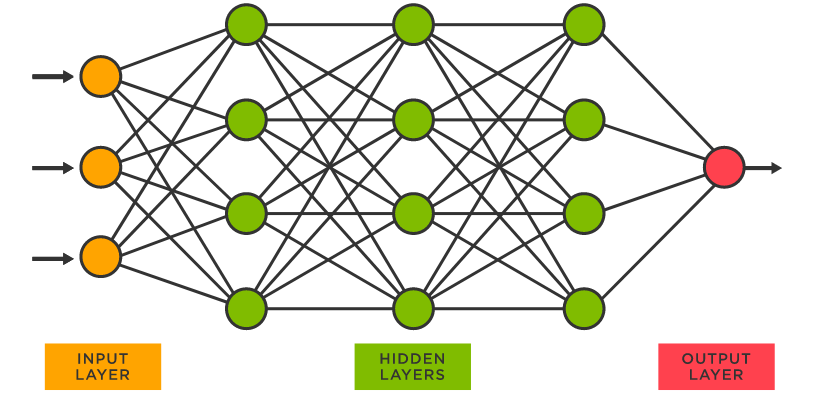
Check out the above images for some good visualizations of the different layers. There are a few things of which we should take note. First off, looked at the connections between individual neurons from one layer to the next. This is illustrating the output of one neuron being fed as input into neurons in the subsequent layer. And secondly, notice that the number of neurons in each layer can vary. The number of neurons in the input layer will correspond to the number of feature inputs in the model while the number of neurons in the output layer will correspond to the number of values outputted by your model. Now the number of neurons in each hidden layer is more of an art. Typically, more complex problems will dictate more complex networks in terms of more hidden layers and a greater number of neurons in each hidden layer.
We're not going to be building anything super complex. For one, we're working with tabular data (i.e. data that could basically be formatted as a spreadsheet). You can do a lot of crazy things with neural networks, which is outside of our scope. I'm talking about things like image and video processing, which are some of the biggest applications of neural networks. You ever come across a program that can classify objects in an image or read about an application that detects cancer or some other condition from an X-ray? These were possible programs that were built using neural networks. That said, they still work great for our purposes here.
Now let's look at what's actually going on in one of these neurons. A forewarning, there's a bit of math involved here. Again, I'm showing you this to give you an idea of what's going on under the covers but we won't actually need to worry about any of the math after this as our libraries will abstract a lot of this away.
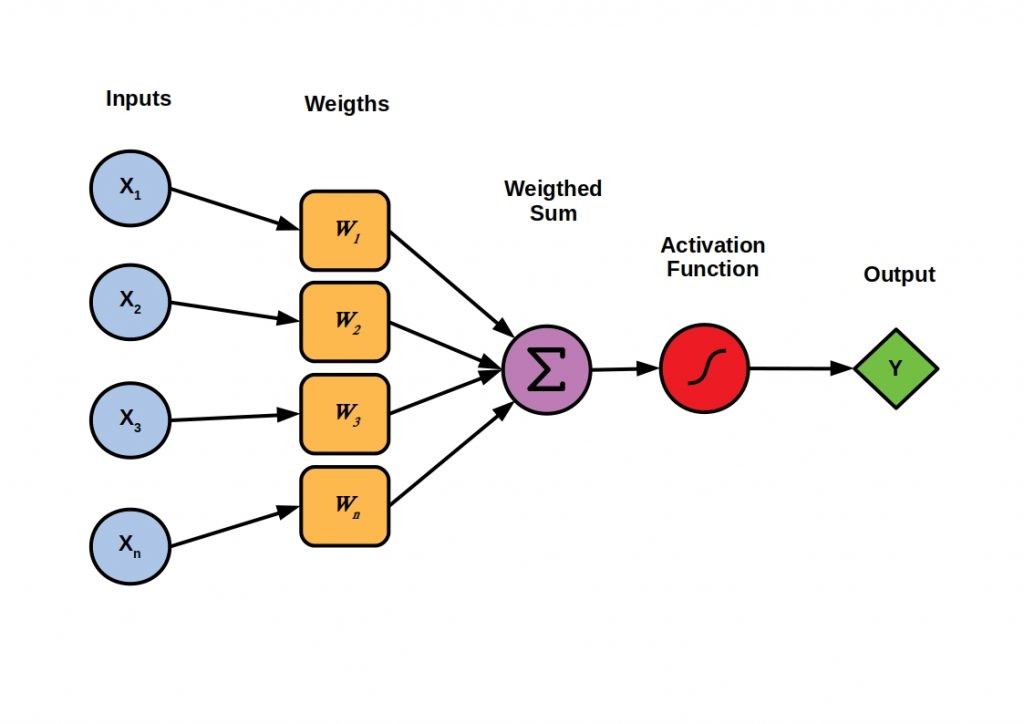
There are all sorts of different neural network architectures and all sorts of different neuron implementations, but we are going pretty basic here. The above diagram illustrates the implementation of a basic type of artificial neuron called a perceptron. As we discussed above, you can see that each neuron takes in a set of inputs, either the feature set of the model (if it's in the input layer) or the output of other neurons in the network. Each input is multiplied by a specific weight and then all of these are summed up. This weighted sum is then passed into an activation function, which is often a type of sigmoid function, but many different types of functions can be used. It is the output of this activation function that is passed to the next layer of neurons as an input, unless the neuron is in the output layer in which case the output of the function is the output of the model.
And that's basically how neural networks work. Again, there are all sorts of architectures and customizations that can be made, but this is a pretty basic architecture to illustrate the basic concepts. So how does this all work in the context of building a model? As with other forms of machine learning, we'll be using training sets to train our neural networks. The basic process will look like this:
- Segregate our training data into a training set and a validation set.
- Construct a blank neural network.
- Connect our blank neural network to our training and validation sets.
- Train the network using a built-in training function.
- Profit.
Obviously, it's a bit more detailed than that, but those are our basic steps. I'd like to draw some attention to step #4, the training step, and how that works with neural networks. Recall the diagram of the artificial neuron up above, particularly the part where inputs are multiplied by a set of weights. Were you wondering where those weights came from? Well, those weights are what are constantly tweaked during training. The training function will iterate through the training set and continuously tweak the weights on each neuron in order to make the model more accurate. We care about accuracy against both our training set as well as against our validation set of data. Note that the validation set does not get used by the training algorithm other than to validate its output. So why do we need a separate validation set anyway? Why not just validate everything on the training set? It's probably time to explain two very important concepts, not just for training neural networks but for any sort of machine learning: overfitting and underfitting.
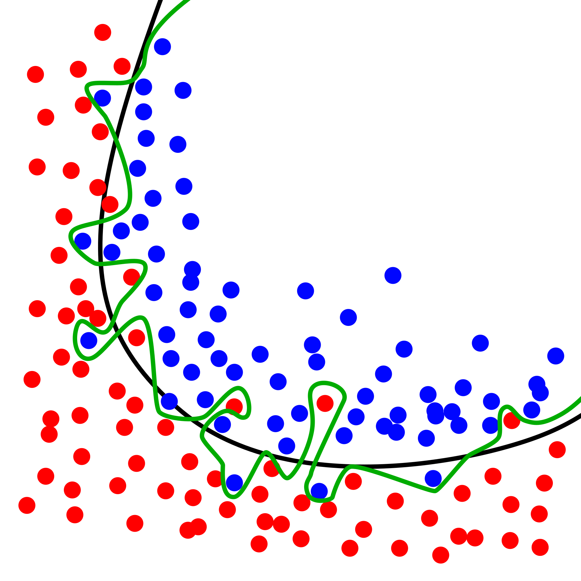
Let's say that we start training our neural network, but we let the training go on indefinitely. What eventually happens is that the model becomes so good at predicting outcomes from the training set that it basically memorizes the training set, which means it can near-perfectly make predictions on data in the training set, but not so much for any new and unfamiliar inputs it may receive. This would be a pretty useless model if it can't really predict anything outside of its training set with any accuracy. We call this overfitting our model.
In contrast, it's entirely possible to not train our model so little that it never gets to a level where it is sufficiently predictive on any sort of data set. This is called underfitting. We want to train our neural networks, but just enough where we are in the sweet spot such that we avoid underfitting without starting to overfit. This is where the validation set comes into play. As we are training a model, we constantly compare its accuracy against the validation set. As long as accuracy against the validation set keeps improving, we are good to continue training. Once accuracy against the validation set starts to deteriorate, we are starting to overfit on the training set, so we want to cut training off before this starts to happen.
So that's the basic rundown on how neural networks work. If you are a little lost in the terminology, hopefully things will start to make more sense once we dive into some code. Like I said before, a lot of this will be abstracted away by the libraries we end up using. There are some other concepts that will come into play, but we'll tackle those as we are coding up our models. Ready to dive in?
Building a Neural Network
We are going to be building a very simple neural network to predict the final scoring margin of college football games. We'll also be using a fairly small set of features, only six inputs to be precise. Normally, you'll have a much larger set of inputs. For comparison, my own model in the CFBD Computer Pick'em Contest is a neural network that is typically composed of upwards of 50 different inputs.
I should emphasize that more features are not necessarily better. There is definitely an art to feature selection and as you build models you'll want to do a fair amount of trial and error. While some data points enhance and improve the accuracy of your model, you'll find that others just add noise and actually drag down accuracy. Anyway, as with most of these articles, we're not concerned with getting a perfect and accurate result. We'll be using just enough features to illustrate the basic concepts. How you apply those concepts in your own real-world modeling will be up to you.
One more thing before diving in. This is the last thing, I promise. Remember the libraries I mentioned earlier that abstract away a lot of the nitty-gritty of building neural networks? The main library we'll be using is called fast.ai, which is built on top of another prominent machine learning library called PyTorch. It providers many abstractions and templates, which means we don't have to spend much time getting into the math or neural network architecture and can spend more time training and fine-tuning our models. There certainly are benefits to getting your hands dirty in the implementation, namely the ability to tweak and customize, but those tasks are overkill for our purposes and fast.ai will do just fine. They also have their own set of machine learning courses which are pretty good. Definitely check them out if this interests you.
Anyway, if you are using my custom container image for data science, then you already have everything you need to get started. If you do not, well... I'll leave it to you to figure out the fast.ai installation, but I believe a simple "pip install fastai" will suffice. Please note that while a lot of machine learning tasks require fast hardware including a dedicated GPU, nothing we are doing here is all that intensive so just about any decent hardware will suffice, even if you are running on a laptop.
Assuming you have Jupyter running and a new Python notebook opened up, let's create our first code block in which we'll organize all of our library imports.
import cfbd
import numpy as np
import pandas as pd

from fastai.tabular import *
from fastai.tabular.all import *
In addition to our typical imports (cfbd, numpy, and pandas), note the import of submodules from the fastai library. Notice that, in particular, we are planning to use the fastai submodules that deal with tabular data. There are other submodules that deal with image processing and more complex tasks, but all of our data will be in tabular format so those are the functions we will need. After running the import statements, you may get what looks like an error message similar to this:

This is nothing to be concerned about. It's looking for a GPU that has been configured to perform more intensive machine learning tasks. We are not doing such tasks so we can safely ignore this message. Next, let's set up our cfbd client.
configuration = cfbd.Configuration()
configuration.api_key['Authorization'] = 'your_api_key'
configuration.api_key_prefix['Authorization'] = 'Bearer'

api_config = cfbd.ApiClient(configuration)
Don't forget to paste your CFBD API key into the above snippet. I also like to set up some of the cfbd submodules that I frequently find myself using. We may not use all of these, but I have a notebook template that includes these by default.
teams_api = cfbd.TeamsApi(api_config)
ratings_api = cfbd.RatingsApi(api_config)
games_api = cfbd.GamesApi(api_config)
stats_api = cfbd.StatsApi(api_config)
betting_api = cfbd.BettingApi(api_config)
We now need to start thinking about features and what data we want to pull. Since we are looking to predict final game margins, I'm going to just go ahead and query all base game data going back to the 2015 season. Why 2015? I don't know. It's pretty arbitrary and I feel like it's a big enough sample to give us a good dataset. I'm also going to pull in current season games (2021), not for training or validation but so that we can make some predictions after the fact. Let's go ahead and also grab betting lines while we are at it.
games = []
lines = []

for year in range(2015, 2022):
    response = games_api.get_games(year=year)
    games = [*games, *response]

    response = betting_api.get_lines(year=year)
    lines = [*lines, *response]
If you're a regular reader of this Talking Tech series, I bet you know what we're going to do next. Let's do some filtering. Notably, we're going to filter down to games that are completed and involve only FBS teams. As of this writing, the CFBD API will return a null or None conference value for FCS and other non-FBS teams. I note this because this is likely to change in the future. But right now, we can exclude games where either team doesn't have a conference. I will also filter out games where there isn't a score value for each team since there isn't yet a public game_status field to denote completed games (I really should get on that).
games = [g for g in games if g.home_conference is not None and g.away_conference is not None and g.home_points is not None and g.away_points is not None]
len(games)
That returned over 4500 games. That's a pretty good sample for our purposes. Let's take a look at which data is included on the game object.
games[0]
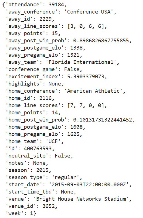
Before converting over to a data frame, I always prefer to whittle the object down to the data points that I actually care about. For this, I'm thinking I'll keep the pregame Elo ratings, conference labels, and points scored for each team, as well as some other data points like year, week, and the neutral_site flag.
games = [
    dict(
        id = g.id,
        year = g.season,
        week = g.week,
        neutral_site = g.neutral_site,
        home_team = g.home_team,
        home_conference = g.home_conference,
        home_points = g.home_points,
        home_elo = g.home_pregame_elo,
        away_team = g.away_team,
        away_conference = g.away_conference,
        away_points = g.away_points,
        away_elo = g.away_pregame_elo
    ) for g in games]

games[0]
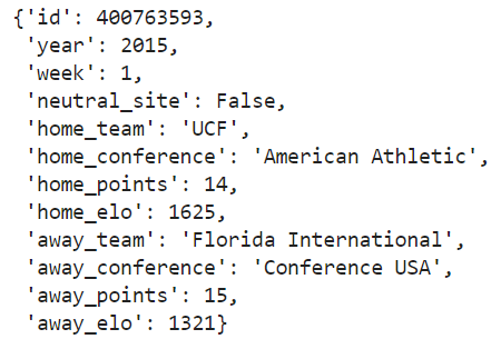
Now, that's more like it. Let's look at the game lines object.
lines[0]
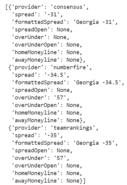
You can see that we potentially have several different line providers for each game. Let's loop through each game object and see if a consensus line exists. If so, we'll add the consensus spread as the spread to our game objects.
for game in games:
    game_lines = [l for l in lines if l.id == game['id']]

    if len(game_lines) > 0:
        game_line = [l for l in game_lines[0].lines if l['provider'] == 'consensus']

        if len(game_line) > 0 and game_line[0]['spread'] is not None:
            game['spread'] = float(game_line[0]['spread'])
We'll also filter games out of our games data set that did not have a consensus spread.
games = [g for g in games if 'spread' in g and g['spread'] is not None]

len(games)
Looks like that didn't take out many games, maybe a hundred or so. Before we go further, I'd like to point something out about betting line data and using them as training features. There's a segment of the CFB analytics Twitterverse that frowns upon using betting line data as training features. I'm talking about the super-duper serious data science snobs. Why is that? I honestly have no clue. Maybe they think it's less pure or cheating or some other non-sensical reason. Do I use betting line data in my own models? It depends. Does it improve the accuracy of what I'm trying to get my model to predict? Then absolutely. What I'm getting at here is that there are old, crusty, data science types out there that may frown upon this practice, but screw them. It's your model, so you build it how you want. As I've said, you'll find that not all data points improve model accuracy. In fact, some detract from it. But if you find a data point that improves the accuracy of your model, then you go for it, no matter what some elitist might say.
Anyway, my apologies for the mini-rant. Let's continue on. Okay, so what are we trying to predict here? The final score margin of games? We should probably go ahead and calculate that on our game objects.
for game in games:
    game['margin'] = game['away_points'] - game['home_points']
Now we're ready to load these bad boys into a data frame and get cooking.
df = pd.DataFrame.from_records(games).dropna()
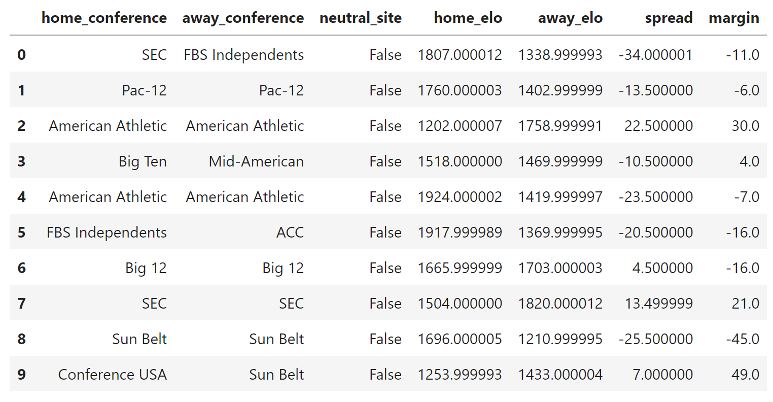
df.head()
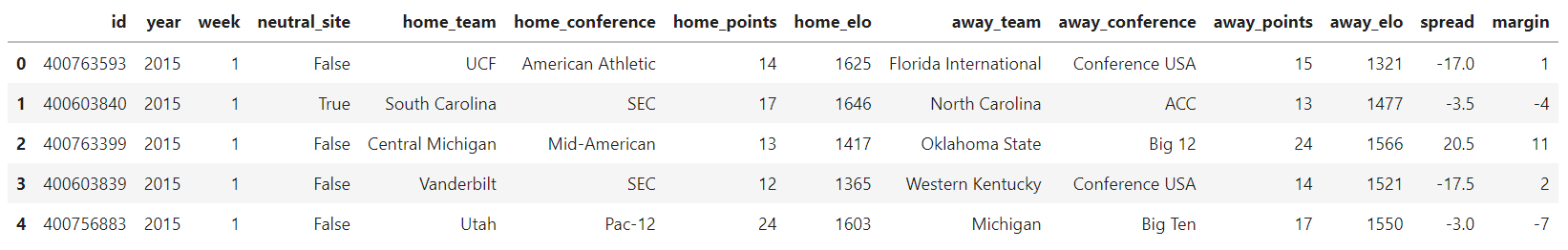
Next, I would like to split this data frame into two separate data frames. Notably, I'd like to separate game data that corresponds to the current season (2021). I'd like to use this data frame later on to compare predictions from our model to real-world results on the field.
test_df = df.query("year == 2021")
train_df = df.query("year != 2021")
The next thing we need to do is think about the training features of our model and how they are categorized. First of all, we have several fields that are not part of the model, but we kept them in the data frame because they have utility in describing our data or they involve the actual expected output of our model. These are fields like game id, year, week, home team, away team, and margin. Next, we have data fields that can be described as categorical data. In other words, they are non-numeric. These are fields like home conference, away conference, and the neutral site flag. True, the neutral site flag could be represented numerically as a 1 or a 0, but we'll leave it as categorical for now. Every other field can be described as continuous, or numerical, data.
excluded = ['id','year','week','home_team','away_team','margin', 'home_points', 'away_points']
cat_features = ['home_conference','away_conference','neutral_site']
cont_features = [c for c in df.columns.to_list() if c not in cat_features and c not in excluded]

cont_features
Our only continuous features ended up being home Elo rating, away Elo rating, and spread. Yes, it probably would have been simpler to manually define these labels and then calculate the excluded labels in contrast to this code snippet, but remember what I said about feature sets typically being much, much larger than this. I usually find continuous features to be the largest set of fields in my data frames, so it's usually easier to define what is excluded rather than what I'm including. It also allows me to tinker by flagging certain fields as excluded in order to see what it does to my model accuracy.
It's time to start using the fast.ai library. The first convenience function we are going to use is RandomSplitter. What this does is randomly split our data set into training and validation sets. We can specify what percentage of the data should be held back as the validation set and RandomSplitter will return the data frame indexes that should belong in each set.
splits = RandomSplitter(valid_pct=0.2)(range_of(train_df))
splits
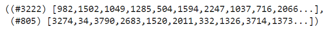
You can see that I specified 20% of rows in the data frame to be held back in the validation set. And RandomSplitter did indeed specify 805 random indexes for inclusion in the validation set with 3222 indexes left to be used in training. This brings us to our next fast.ai convenience object, TabularPandas. TabularPandas defines how our data is pre-processed before it is compiled into a data loader that can be read by our neural network during training.
to = TabularPandas(train_df, procs=[Categorify, Normalize],
                    y_names="margin",
                    cat_names = cat_features,
                    cont_names = cont_features,
                   splits=splits)
Let's walk through what's going on there. We're first passing in the data frame consisting of all our training data. Next, we're passing in an array of predefined procs, Categorify and Normalize. Categorify will preprocess our categorical data into numeric data that our model can understand. Normalize will normalize our continuous data into a range that our model can understand. For example, some neural networks can only process data between 0 and 1 or between -1 and 1. Normalize takes care of this for us. Lastly, there are other procs we are not using that could be useful, such as FillMissing. Had we not dropped games with missing data, we could have used the FillMissing proc to fill in missing inputs using the mean value of the input or some other mechanism.
The y_names parameter is used to denote the name of our output or outputs. We have a single expected output here, margin. cat_names and cont_names are just the names of our categorical and continuous data fields. Lastly, the splits parameter is used to pass in the output of RandomSplitter, telling the preprocessor how data should be segregated into training and validation sets.
Let's load this all into a data loader.
dls = to.dataloaders(bs=64)
dls.show_batch()
The bs parameter defines batch size, which is the number of samples that will be processed in a given batch. If you find you are running into memory or other issues in subsequent steps, you can feel free to adjust this number.
We can now create our first neural network!
Remember when we went through all the stuff about neural network architecture and I said that we really wouldn't need to worry about most of it later on? The fast.ai library has predefined neural network architectures that are optimized for various things. It just so happens that they have a template that is optimized for tabular learning. It's pretty easy to use.
learn = tabular_learner(dls, metrics=mae, lr=10e-1)
Now, I think it's mostly self-explanatory what's going on in that single line of could, but I'm sure you have questions about the parameters that were passed in. Let's step through those. First, we passed in our data loader object. Next, we used the metrics parameter to tell our training function what type of metric we want to use to judge the accuracy of our model. There are several different predefined metrics based on the type of learning you are doing. Some of them cover regression and others are geared towards classification. We're doing regression here and my preferred metric is mean absolute error, or MAE, but you can choose another if you like. The last parameter, lr, concerns learning rate, the rate at which our model will learn and adjust itself during training. Let's dig into that some more.
Learning rate is exactly what it sounds like, the rate at which adjustments are made to our model during the training process. It seems logical that we would want to amp that up super-high. I mean, more learning is good, right? Well, that's actually not as logical as it may seem. Remember our discussion on overfitting and underfitting? What's going to happen if we set our learning rate too high? That's right, it's going to quickly overfit on our training set and not be of much use for anything else. Conversely, setting the rate too low will lead to underfitting. We want to find that sweet spot that will get our model just right while avoiding both of these pitfalls.
You're probably wondering how we go about picking an initial learning rate. Another convenient method provided by fastai is lr_find, which is meant to help find the ideal rate to optimize our training. Let's check it out.
learn.lr_find()
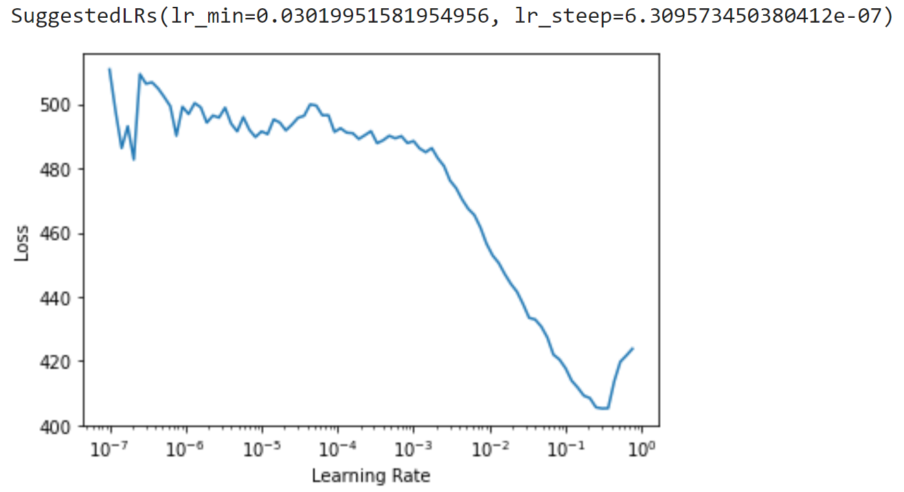
Let's break down this output, starting with the graph. The graph plots various learning rates against training loss. Loss is basically how accurate our model is as making predictions, the less loss the better. Looking at the graph, we want to pick a point at which the amount of loss is decreasing, ideally where the graph is sloping down the most. Notice that we have a pretty consistent downward slope starting around a learning rate of 10-3 and continuing to just past 10-1? We'll pick a learning rate smack dab in the middle of that range. We could go with 10-2. You see that fastai actually suggests a few learning rates for us, one of which (lr_min) is actually in the middle of our range. The other (lr_steep) is actually at the extreme left of the graph where there is a lot of noise and is certainly just that, noise.
Depending on which rate you chose, we can now plug this in and train our neural network.
learn = tabular_learner(dls, metrics=mae, lr=10e-2)
learn.fit(10)
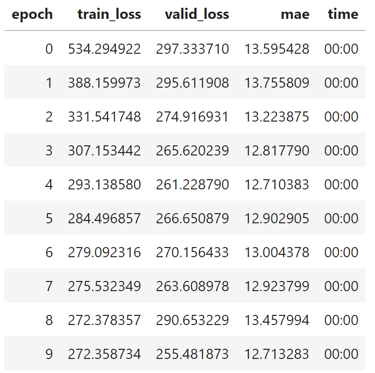
We're going to be doing some trial and error here. I always start off instantiating a fresh network and running the training function with an arbitrarily high number of epochs, like 10. We are still not out of the woods when it comes to overfitting and underfitting. We picked a good learning rate, but that's just one part of the puzzle. We now need to hit the right number of training epochs. Let's break down this chart. Each epoch has three columns that we care about:
- train_loss is the amount of loss measured on our training set. We want this to be as low as possible while not overfitting.
- valid_loss is the amount of loss measured on our validation set. We also want this to be as low as possible. If it's too high, then our model is underfitted.
- mae is the metric we specified earlier for measuring the predictive accuracy of our neural network, mean absolute error. I probably don't need to repeat, but we also want this to be as low as possible.
So how do we know when to cut off training for optimal results? There are a few things I look at in this chart to determine the optimal number of training epochs.
- Training loss, validation loss, and the predictive metric (MAE here) are all still going downward.
- The difference between training loss and validation loss is as small as I can get it. This means we have an optimal fit.
- If anything, training loss should be slightly higher than validation loss. Otherwise, we run into potential overfitting.
Going by this criteria, I'd put the optimal number of training epochs at around 5 since MAE starts to increase after that. Validation loss also starts to increase shortly thereafter. Let's go ahead and re-run the learning function with 5 epochs.
learn = tabular_learner(dls, metrics=mae, lr=10e-2)
learn.fit(5)
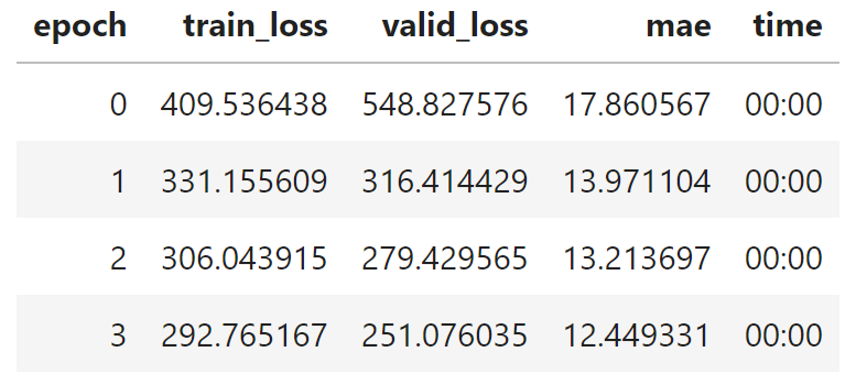
I'll actually re-run this block of code several times. You'll notice that results can vary from run to run, so I'll typically re-run it until I get a result that I like. You can see that the above screenshot doesn't match the code block because only 4 training epochs are pictured instead of the 5 in the code block based on my own trial and error. Your own results may vary. At any rate, it looks like we have our model trained to a predictive accuracy of 12.4 on the validation set, which is actually pretty dang good! I'm actually surprised we got it down that low with our small feature set, but I guess it goes to show that sometimes less is more and more features can just add noise instead of value.
We can actually check out the output of our model on the training data.
learn.show_results()
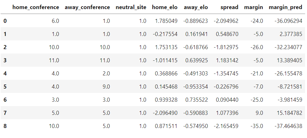
Here, we're comparing the margin column, which denotes the real-world final score margin, with margin_pred, our trained neural networks predicted margin. Not too bad! I don't think it's going to beat Vegas, but not bad for a start at all.
Making Predictions
Our neural network is fully trained and we now have everything we need to begin making predictions. In order to do so, we just need a data frame that is in the same format as our initial data frame that we feed into our data loader. If you recall, we actually partitioned that data frame and held back games from the current season (2021). I believe this test data frame has current season games that have already been played, but obviously we would be running this on games that have not been played were we doing this for real and not just for demo purposes.
Anyway, here's the code block to load predictions into our test data frame of 2021 data.
pdf = test_df.copy()
dl = learn.dls.test_dl(pdf)
pdf['predicted'] = learn.get_preds(dl=dl)[0].numpy()
pdf.head()
We first make a copy of our test data frame that we can load into our neural network. On line 2, we create a data loader of our test data using the same configuration as our initial training and validation sets. Lastly, we use the learner to get predictions for all rows and load this into a new data frame column.
In real-world scenarios, I typically like to compare my model output to the spread to get a good gauge of things. You can call this an eye test of sorts just to make sure we're getting output that is at least reasonable.
pdf[['home_team','away_team','spread','predicted']].round(1)
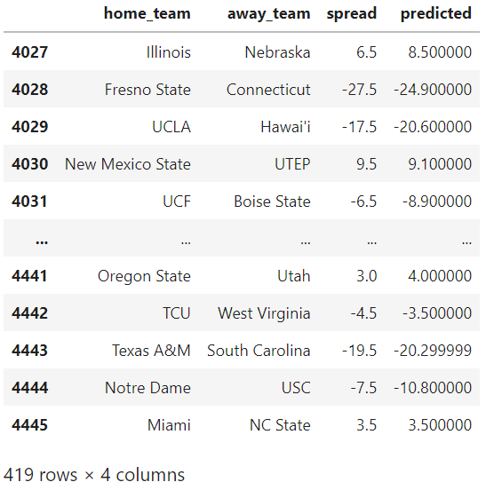
That all looks pretty reasonable to me. Again, I doubt it's going to consistently beat Vegas, but it's not too bad for this demonstration.
The last thing we should do is export our model so that we can load it up and use it later. This will allow us to safely shut down Jupyter without fear of losing any of our work. I'm going to name my model file "talking_tech_neural_net", but you can pick whichever name you like.
learn.export('talking_tech_neural_net')
Now next time we want to load up and use our model again, we can use the load_learner method to restore it and make more predictions.
learn = load_learner('talking_tech_neural_net')
Going Further
Congrats! You have successfully trained your first artificial neural network!
As we talked about, there are several ways this can be improved, largely centered around training features. We only used a small handful of features in our training set, but you'll typically want many more inputs. Like I said earlier, my own game prediction models usually have around 50 or so different data points. So what data points can we add to this to make it more predictive? With the CFBD Python library, there are a wealth of different data points that can be explored. And remember, not all data points add value; some just add noise. I'll leave it up to you to tinker around and figure out which features are best for predicting game outcomes.
Lastly, what other applications do you think neural networks can have? What are CFB-related things can we try to predict? Are we limited to regression-type problems like this or are there any classification problems we can try to solve? Again, I leave it all up to you.
I hope you enjoyed this post and got something out of it. This is a post I have been planning to write for quite some time and am ecstatic to finally be able to share it with you. As always, give me a holler if you end up using this walkthrough to build anything super cool. I always love seeing what people come up with, so please do share with us whether you are on Twitter (@CFB_Data), the CFBD Discord server, /r/CFBAnalysis, or wherever else.