Programming

Opponent Adjusted Stats Using Ridge Regression

Bud Davis

Oct 12, 2021 • 10 min read

"The biggest variable in football is the fact that each team plays a different schedule against teams of disparate quality." - Football Outsiders

"They ain't played nobody Pawllllllll." - SEC Proverb, author unknown

Motivation

One of the interesting quirks of football is that some statistics are more reflective of the quality of your opponent than they are of your own team. This is where opponent-adjusted stats can be very helpful.

At its most basic level we want to perform an opponent adjustment that solves for a given stat by taking into account the quality of both the offense and the defense. Now there are a number of ways you could get at this. My preferred method (GitHub) is derived from the methodology laid out for here¹ and here² for college basketball stats. Before we get into that method, let's talk about the most common type of opponent adjustment you'll see, which involves averaging:

Averaging Method

The most basic type of opponent adjustment is to use averaging. With averaging, you could quantify how Team A did against Team B, by comparing Team A's performance vs Team B against Team B's average against all other opponents.

An example: Team A gave up 9.4 yards per pass attempt (YPA) in a single game against Team B. In a vacuum, 9.4 YPA might lead you to believe Team A has a poor pass defense. But when you consider that Team B averaged 10.7 YPA against all other opponents, suddenly 9.4 YPA looks a lot better. In fact, this performance by Team A was 1.3 YPA better than average! Team A was 2019 Clemson and Team B was the 2019 LSU.

The shortcoming of an averaging method is that it only deals with one side of the ball and it requires multiple iterations. In the above example, we got an estimate of how good Clemson's defense was relative to LSU's offense. So let's say we did an opponent adjustment for all of the offenses Clemson faced (i.e., we calculate a season's worth of residuals like the 1.3 YPA above). Then we'd have a nice first-pass estimate of the quality of Clemson's defense. We could do this for all FBS defenses to get an opponent-adjusted measure of defense quality. But then we should flip the problem, and adjust offenses relative to this adjusted defensive quality measure. This would in turn give us a new measure of offense quality... which we could then do another round of defensive adjustments on... you can see where this is going, we're stuck in a loop of iteratively averaging back and forth. In the above-linked video, the Youtuber recommends four (!!!!) rounds of offensive and defensive adjustment before the stats stabilize to a useful opponent-adjusted metric. Luckily, there is a much more efficient, robust, and easier method to perform opponent adjustments.

Ridge Regression Overview

Rather than iteratively adjusting our stats for offense and defense, it's easier to set up a single equation with offense and defense as variables of interest, and solve for both simultaneously in a multivariate regression^1,2. The basic idea is that the stats we're interested in can be approximated as a function of the quality of the offense, the quality of an opposing defense, and home-field advantage:

Equation 1: EPA ~ OffenseQuality + DefenseQuality + HomefieldAdvantage + Constant

Ridge Regression provides an elegant method to solve Equation 1. Ridge Regression is a special form of regression that uses L2 regularization to apply a penalty term (lambda/alpha) to the square of the coefficients (helpful video link). This penalty term: (1) helps reduce any potential issues associated with multicollinearity and (2) produces more reasonable values for each team-coefficient than an ordinary Least Squares regression. We can tune this penalty hyperparameter using the built-in Ridge Cross-Validation module. Overall, Ridge Regression provides a method that simultaneously solves for offense and defense, is statistically robust, reduces issues with multicollinearity, and produces reasonable estimates of opponent-adjusted team quality

Code Overview

The below code can be found at my GitHub.

Part 1 - Configure Inputs

First, we need to load in load in our modules, choose what year we're interested in, configure our CFBD API key, and create some empty data frames to be filled. For this example, we will look at 2019 data.

### -------------------------------------------------------------------------
### PART 1 - Configuration
### -------------------------------------------------------------------------
# @jbuddavis
# https://github.com/jbuddavis

# Load modules
import pandas as pd 
import time
import cfbd
from sklearn import linear_model

# track time to complete, turn off pandas warning
start = time.time()
pd.options.mode.chained_assignment = None

#%% Configure Inputs
# Choose what year you would like to perform adjustment on
year = 2019 # year of interest

# Configure API key authorization
configuration = cfbd.Configuration()
configuration.api_key['Authorization'] = 'YOUR_API_KEY_HERE'
configuration.api_key_prefix['Authorization'] = 'Bearer'

# create empty dataframes to be filled
dfCal = pd.DataFrame() # dataframe for calendar
dfPBP = pd.DataFrame() # dataframe for pbp data
dfGame = pd.DataFrame() # dataframe for game information
dfTeam = pd.DataFrame() # dataframe for team information

Part 2 - Ping the API

Next, we ping the CFBD API to get our data. First, we get the calendar to guide the rest of our requests. Then we get the Play-by-Play (PBP) and Game Information for each week. Then we also get a dataframe of FBS schools

### -------------------------------------------------------------------------
### PART 2 - Ping the API
### -------------------------------------------------------------------------
# get calendar for season
api_instance = cfbd.GamesApi(cfbd.ApiClient(configuration))
api_response = api_instance.get_calendar(year)
dfCal = pd.DataFrame().from_records([g.to_dict()for g in api_response])

# loop through the calendar and get the PBP for each week
print('Getting PBP data for year '+str(year)+'...')
for i in range (0,len(dfCal)):
    # iterate through calendar to get variables to pass to the API
    week = int(dfCal.loc[i,'week']) # get week from calendar
    season_type = dfCal.loc[i,'season_type'] # get season type from calendar
    # Get play-by-play Data
    api_instance = cfbd.PlaysApi(cfbd.ApiClient(configuration))
    api_response = api_instance.get_plays(year,week,season_type=season_type)
    dfWk = pd.DataFrame().from_records([g.to_dict()for g in api_response])
    dfPBP = dfPBP.append(dfWk)
    # Get game info (used for homefield advantage)
    api_instance = cfbd.GamesApi(cfbd.ApiClient(configuration))
    api_response = api_instance.get_games(year, week=week, season_type=season_type)
    dfGameWk = pd.DataFrame().from_records([g.to_dict()for g in api_response])
    dfGame = dfGame.append(dfGameWk)
    print('PBP data downloaded for '+season_type+' week',week)

# Get FBS teams
api_instance = cfbd.TeamsApi(cfbd.ApiClient(configuration))
api_response = api_instance.get_fbs_teams(year=year) 
dfTeam = pd.DataFrame().from_records([g.to_dict()for g in api_response])
dfTeam = dfTeam[['school']]
dfTeam.to_csv('teams.csv',index=False) #print FBS teams to csv

Part 3 - Format the data

Next, we need to format the data. I've found that dropping FBS vs FCS games helps produce more reasonable results. We also need to drop plays where the EPA (ppa) is undefined. For home-field advantage (HFA) we assign a value of 1 for the home team on offense, -1 for the away team on offense, and 0 for neutral site games.

I like to go ahead and output the formatted PBP data to a .csv now (allPBP2019.csv). This helps save time in case you want to tweak the Opponent Adjustment portion of the code because there is no need to reload all the data from the API.

### ------------------------------------------------------------------------
### PART 3 - Format the data
### -------------------------------------------------------------------------
print('Formatting data...')

# Drop non-"fbs-vs-fbs" games
dfPBP = dfPBP[dfPBP['home'].isin(dfTeam.school.to_list())] 
dfPBP = dfPBP[dfPBP['away'].isin(dfTeam.school.to_list())] 
dfPBP.reset_index(inplace=True,drop=True)
dfGame = dfGame[dfGame['home_team'].isin(dfTeam.school.to_list())]
dfGame = dfGame[dfGame['away_team'].isin(dfTeam.school.to_list())]
dfGame.to_csv('games'+str(year)+'.csv', index=False) # print game data to csv 
dfGame.reset_index(inplace=True,drop=True)   

# drop nas
dfPBP.dropna(subset=['ppa'],inplace=True)
dfPBP.reset_index(inplace=True,drop=True)

# create list of neutral site games
neutralGames = dfGame['id'][dfGame['neutral_site']==True].to_list()

# All Plays
df = dfPBP[['game_id','home','offense','defense','ppa']] #columns of interest
df.loc['hfa'] = None # homefield advantage
df.loc[(df.home == df.offense),'hfa']=1 # home team on offense
df.loc[(df.home == df.defense),'hfa']=-1 # away team on offense
df.loc[(df.game_id.isin(neutralGames)),'hfa']=0 # neutral site games
df = df[['offense','hfa','defense','ppa']] # drop unneeded colums
df.dropna(subset=['ppa'],inplace=True) # drop nas
df.reset_index(inplace=True,drop=True) # reset index
df.to_csv('allPBP'+str(year)+'.csv',index=False) # output to csv

print('Data formatted')

Part 3.5 - Check Out Our Dataframe

Let's look at how our dataframe is formatted really quick:

In[1]: df.head()
Out[1]: 
   offense  hfa  defense       ppa
0  Alabama  0.0     Duke -0.514220
1  Alabama  0.0     Duke -0.227265
2  Alabama  0.0     Duke -0.337948
3     Duke  0.0  Alabama -1.383841
4     Duke  0.0  Alabama -0.148933

Part 4 - Initialize Opponent Adjustment

Here we will read in our PBP csv and initialize some of the variable names before we continue with the opponent adjustment. Usually, this part is important for when I perform the opponent adjustment as part of a callable function, but for this example, it's easier for you to play with (and understand) the code if it's written sequentially. The main thing we need to do here is to make sure the variable names that will be used in the adjustment match our dataframe column names. If you want to see how opponent adjustment can be executed as a callable function, check out my code here.

### -------------------------------------------------------------------------
### PART 4 - Initialize Opponent Adjustment
### -------------------------------------------------------------------------
# if you just need to tweek the opp-adj func, to save time, after the first 
# round of pbp downloading, comment out the above code & read in the pbp csvs 
dfTeam = pd.read_csv('teams.csv')
df = pd.read_csv('allPBP'+str(year)+'.csv')

# dataframe column names to help guide opponent adjustment function
offStr = 'offense' # Column of interest, the team/player we want to adjust
hfaStr = 'hfa' # Homefield Advantage column name
defStr = 'defense' # Opponent column name
stat = 'ppa' # stat to adjust on

Part 5a - Perform Opponent Adjustment

First, we make dummy variables for all the offenses & defenses in our dataframe. Then we set up the regression equation using these 261 dummy variables (HFA + Off/Def for 130 teams) as inputs and the df['ppa'] column as the target variable. We use Ridge's Cross-Validation functionality to search out a reasonable alpha/lambda penalty parameter. Alpha will usually be around 175 for full-season data but can be much higher for partial-season datasets. Once we have a good value for alpha, we perform the regression on the data.

### -------------------------------------------------------------------------
### PART 5 - Perform Opponent Adjustment 
### -------------------------------------------------------------------------
# loop through our list of dataframes & adjust each for opponent & homefield advantage
print('Performing Opponent-Adjustment...')

# Create dummy variables for each Team/Opponent, plus Homefield Advantage
dfDummies = pd.get_dummies(df[[offStr, hfaStr, defStr]])

# Hyperparameter tuning for alpha (aka lambda, ie the penalty term) 
# for full season PBP data, the alpha will be 150-200, for smaller sample sizes it may find a higher alpha
rdcv = linear_model.RidgeCV(alphas = [75,100,125,150,175,200,225,250,275,300,325], fit_intercept = True)
rdcv.fit(dfDummies,df[stat]);
alf = rdcv.alpha_

# Or set Alpha directly here
# alf = 175

# Set up ridge regression model parameters
reg = linear_model.Ridge(alpha = alf, fit_intercept = True)  

# Run the regression
# X values in the regression will be dummy variables each Offense/Defense, plus Homefield Advantage
# y values will be the raw value from each game for the specific stat we're adjusting
reg.fit(X = dfDummies, y = df[stat])

Here is what the dummy variables look like:

In[1]: dfDummies.columns
Out[1]: 
Index(['hfa', 'offense_Air Force', 'offense_Akron', 'offense_Alabama',
       'offense_Appalachian State', 'offense_Arizona', 'offense_Arizona State',
       'offense_Arkansas', 'offense_Arkansas State', 'offense_Army',
       ...
       'defense_Virginia', 'defense_Virginia Tech', 'defense_Wake Forest',
       'defense_Washington', 'defense_Washington State',
       'defense_West Virginia', 'defense_Western Kentucky',
       'defense_Western Michigan', 'defense_Wisconsin', 'defense_Wyoming'],
      dtype='object', length=261)

Part 5b - Run the Regression

Once we run the regression, we have a fair amount of formatting to get the regressed coefficients in a nice format for us to work with. We need to add back in the intercept to get an adjusted value. We use the coefficient names to split our adjusted offense and defensive values into separate dataframes with their associated team name. We also print the home-field advantage and alpha value to the terminal for QA/QC. For 2019, home-field advantage was roughly 0.018 EPA/play!

NOTE: HFA will be higher for passing than rushing.

# Extract regression coefficients
dfRegResults = pd.DataFrame({
    'coef_name': dfDummies.columns.values,
    'ridge_reg_coef': reg.coef_})

# Add intercept back in to reg coef to get 'adjusted' value
dfRegResults['ridge_reg_value'] = (dfRegResults['ridge_reg_coef']+reg.intercept_)

#Print the HFA and Alpha values
print('Homefield Advantage: (alpha: '+str(alf)+')')
print('{:.3f}'.format(dfRegResults[dfRegResults['coef_name'] == hfaStr]['ridge_reg_coef'][0]))

# Offense
dfAdjOff = (dfRegResults[dfRegResults['coef_name'].str.slice(0, len(offStr)) == offStr].
   rename(columns = {"ridge_reg_value": stat}).
  reset_index(drop = True))
dfAdjOff['coef_name'] = dfAdjOff['coef_name'].str.replace(offStr+'_','')
dfAdjOff = dfAdjOff.drop(columns=['ridge_reg_coef'])

# Defense
dfAdjDef = (dfRegResults[dfRegResults['coef_name'].str.slice(0, len(defStr)) == defStr].
   rename(columns = {"ridge_reg_value": stat}).
  reset_index(drop = True))
dfAdjDef['coef_name'] = dfAdjDef['coef_name'].str.replace(defStr+'_','')
dfAdjDef = dfAdjDef.drop(columns=['ridge_reg_coef'])

Part 6 - Join Data & Output

Lastly, we just need to aggregate our data for each team. To do this, we just need to join our dfTeam dataframe of all 130 FBS teams. For comparison, I put the raw offensive & defensive EPA/play next to the adjusted EPA/play. For output, I like to round the data to the thousandths place.

### -------------------------------------------------------------------------
### PART 6 - Join Data and Output
### -------------------------------------------------------------------------

# associate the raw and adjusted epa with each team
dfTeam['rawOff'] = dfTeam.join(df.groupby('offense').mean().ppa, on='school').ppa # raw avg ppa
dfTeam['adjOff'] = dfTeam.join(dfAdjOff.set_index('coef_name'), on='school').ppa # adj est ppa
dfTeam['rawDef'] = dfTeam.join(df.groupby('defense').mean().ppa, on='school').ppa
dfTeam['adjDef'] = dfTeam.join(dfAdjDef.set_index('coef_name'), on='school').ppa

# final formatting and output
dfTeam = dfTeam.round(3) # round adjusted value to thousandths 
print(dfTeam)
dfTeam.to_csv('adj'+str(year)+'.csv', index=False)
print('Adjusted Data ouput to: adj'+str(year)+'.csv')
end = time.time()
print('Time Elapsed (s): ',round(end-start,1))

Data QA/QC

Your dataset should look something like this:

In[1]: dfTeam
Out[1]: 
                school  rawOff  adjOff  rawDef  adjDef
0            Air Force   0.307   0.262   0.133   0.124
1                Akron  -0.062  -0.060   0.217   0.249
2              Alabama   0.397   0.378   0.034   0.048
3    Appalachian State   0.259   0.220   0.095   0.115
4              Arizona   0.180   0.179   0.257   0.214
..                 ...     ...     ...     ...     ...
125   Western Kentucky   0.139   0.125   0.087   0.116
126   Western Michigan   0.235   0.183   0.156   0.183
127      West Virginia   0.071   0.106   0.180   0.157
128          Wisconsin   0.295   0.320   0.040   0.028
129            Wyoming   0.153   0.139   0.069   0.117

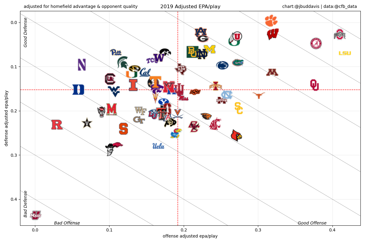
[130 rows x 5 columns]

Or shown graphically:

Conclusions

The above method and code should allow you to calculate opponent-adjusted statistics using Ridge Regression. Please feel free to reach out to me on twitter (@jbuddavis) if you have any problems or issues. If you find this code useful, please give me a shoutout when you use it and star it on GitHub. I can't wait to see what you create and I hope my code/blog was helpful!