
Talking Tech: Creating a Simple Rating System

Welcome back! We didn't get to have much fun last time, as we were mostly concerned with setting up an environment for data analytics in Python. A few people even offered feedback on different tools and setups they use, which is fantastic. Just as there's more than one way to skin a cat, there's several different tools and setups out there that are all equally valid. Someone like myself, who has a background in software engineering, is going to tackle things differently than someone with a more traditional background in data science who in turn may tackle that same thing quite differently from someone who has a different kind of background.
And this is exactly what makes Docker such an indispensable tool. You can try out all sorts of different environments, tools, and configurations within seconds and without having to worry about actually installing anything directly onto your machine. So regardless of setup, Docker is always something I highly recommend as a starting point. Anyway, let's move onto this iteration of Talking Tech.
Computer Rankings?
A very common question that gets asked both on the r/CFBAnalysis subreddit as well as the r/CFBAnalysis Discord server is, "How do I create a computer ranking system?". And as with many questions in this space, there is really no one simple answer or approach. The approaches to computer rankings are as varied as approaches to human polls. It all boils down to what you would like to quantify and how. Do you just care about resume and past results (what we would call retrodictive rankings)? Or perhaps you are looking to do something more predictive, like SP+ which is more concerned on predicting future outcomes? Once you decide on an approach, it becomes a matter of picking which data points to apply. This can include a lot of trial and error.
Personally, I have created several different types of ranking systems over the years across various different programming languages. Heck, you don't even really need to know programming to create your own ranking. This is how my own rankings have evolved throughout the years:
- I started out with a basic system entirely composed of formulas in an Excel spreadsheet.
- A few years later, I wrote a C# program to perform some more complex calculations and export to a spreadsheet.
- A few years after that, I trained a neural network using a JavaScript library using some basic team stats
- Lastly, I trained another neural network using more advanced metrics
These were just the major milestones of my own model. There are always nonstop intermediary steps that involve all sorts of tinkering. Whether you go with a spreadsheet-based model or something more automated, one of the biggest challenges in college football is that not all teams and schedules are created equally. For every Alabama or Clemson, you have a UMass or an Akron and every step in between. And with 130 FBS teams with a 12-game regular season, there is often not a lot of overlap between schedules, especially teams from different conferences and regions. So whatever approach you choose, you'll want to be sure to account for strength of schedule in some way. We'll be going over one such approach in this article.
Introducing SRS
One of the most common answers to queries about building computer rankings from scratch is to start with an SRS system and go from there. SRS, or Simple Rating System, is a rating system pioneered by Pro Football Reference, specifically by Doug Drinen in the Spring of 2006. Doug provided a primer on the system, from which we'll provide an excerpt summarizing the basic idea behind SRS:
The idea is to define a system of 32 equations in 32 unknowns. The solution to that system will be collection of 32 numbers and those numbers will serve as the ratings of the 32 NFL teams.
...
So every team's rating is their average point margin, adjusted up or down depending on the strength of their opponents. Thus an average team would have a rating of zero.
As you can see, SRS is primarily concerned with two data points:
- A team's average scoring margin
- Strength of schedule
It spits out a number that essentially functions as a weighted scoring margin. A team's weighted scoring margin is basically their average margin adjusted up or down for SOS. A team with a final rating of 0 is considered to be completely average whereas a team with a +5 rating is considered to be 5 points better than an average team. Sound familiar? This is pretty much the crux of what Bill Connelly's SP+ ratings attempts to quantify. Now, SP+ doesn't calculate these numbers in quite the same way as SRS. Well that's not entirely true. We don't really know how SP+ spits out those number. We know which factors Connelly incorporates (which are assuredly different from those considered in SRS), but not the manner in which they are used.
Anyway, does that make sense? We haven't really gone over the methodology SRS uses to get this output. Basically, it creates as system of linear equations, one for each team, and solves it. I highly recommend reading through Doug's primer at some point as it goes a little deeper into the math (and it's pretty short). At any rate, we'll be walking through step-by-step how to do this using Python.
Model Building
First thing's first, we need to get our environment up and running. If you are following along from last time, then open up a terminal and enter the following command.
docker run -p 8888:8888 -e JUPYTER_ENABLE_LAB=yesYou may also want to specify a volume mount point in order to save your work. If not, I'll be posting my Jupyter notebook on GitHub shortly. I did add some libraries to the image, namely the Plotly Python library for generating charts down the road. If you have the latest version, you should be good to go. Otherwise, it may take a few minutes to download the latest image.
By this point, you should have Jupyter up and loaded in your web browser of choice, whether you are using the Docker image or not. Go ahead and create a new Python notebook. We'll create our first code block in the notebook and use it to import any libraries we will be using. We'll also configure the CFBD package. If you haven't yet make sure to grab your free API key here.
import numpy as np
import pandas as pd
import cfbd

configuration = cfbd.Configuration()
configuration.api_key['Authorization'] = 'your_api_key'
configuration.api_key_prefix['Authorization'] = 'Bearer'

api_config = cfbd.ApiClient(configuration)
We're going to be creating SRS ratings for the 2019 season, but you should be able to go back and use the same code to generate ratings for prior seasons quite easily after getting through this. Remember, the main two data points that SRS is concerned with are scoring margin and SOS. We'll be calculating the latter as part of the base SRS calculation. As for the former, score data is very easily accessed via the CFBD API's /games endpoint. Let's use Python's request library to load all games from the 2019 season into a pandas DataFrame object.
response = games = cfbd.GamesApi(api_config).get_games(year=2019, season_type='both')

data = pd.DataFrame.from_records([g.to_dict() for g in games])
data.head()
You should get output similar to below. This only outputs the first five games in the data frame, but do you notice anything in those five games?
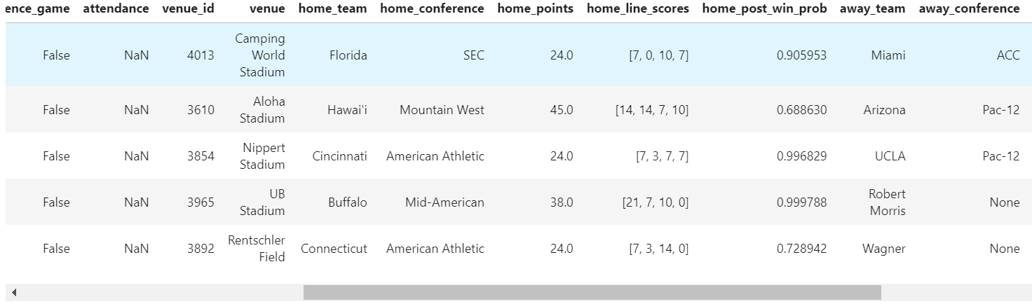
This output includes games against non-FBS opponents. How should we treat such games? There are a few different options. For one, we can just include them but then our system of equations grows much larger and includes teams that offer very few data points. Sports Reference takes the approach of just tossing all non-FBS teams into a bucket and treating them as a single team. I don't really like that much because even still, not all FCS teams are the same. We're just going to exclude them. CFBD has an, admittedly, peculiar way of distinguishing FCS teams. Looking in the conference columns above, you'll see that all non-FBS teams have a null conference value, which Python represents are 'None'. Let's go ahead and filter out any games where either team has no conference data and thus are non-FBS schools.
data = data[
    (pd.notna(data['home_conference'])) #
    & (pd.notna(data['away_conference']))
]
There's still one oddity with which we need to deal. This data could potentially include games that have not yet been played. As I'm writing this, there are still a couple of bowl games left in the 2019 season, including the National Championship game. Another admitted peculiarity of the CFBD API at the time of writing is that it does not have a flag for completed games. Instead, we need to filter out games lacking score data. I'm going to just include these filters with the ones in the snippet above.
data = data[
    (data['home_points'] == data['home_points'])
    & (data['away_points'] == data['away_points'])
    & (pd.notna(data['home_conference']))
    & (pd.notna(data['away_conference']))
]
Next thing I want to do is to find each team's average scoring margin. Notice how we have data frame columns for home points and away points. Let's create new columns for the home and away scoring margins. One question we need to answer, though, is how we deal with home field advantage. The SRS formula used by Sports Reference notably does not make any sort of home field adjustment, but I would still like to make such an adjustment. We'll set home field advantage at +2.5 points for the purposes of this article, but may go back and adjust. The code for these calculations looks like this:
data['home_spread'] = np.where(data['neutral_site'] == True, data['home_points'] - data['away_points'], (data['home_points'] - data['away_points'] - 2.5))
data['away_spread'] = -data['home_spread']
data.head()
What is going on above? Well first off, I am making this calculation conditional on whether the game is at a neutral site. If it's at a neutral site, I include no home field adjustment. Otherwise, I subtract 2.5 points from the home team's margin. The away team's margin is just the inverse of the home team's.
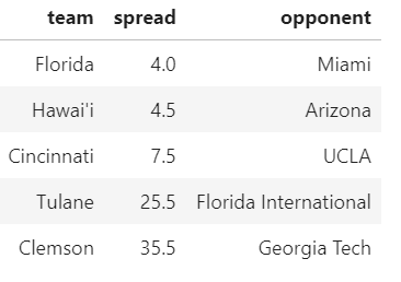
We're going to do a little cleanup here. It would be nice if we could get our data into a format that would make our calculations are little bit easier. I'm thinking of something that just has the following columns:
- team name
- spread
- opponent
To do this, we'll essentially be converting each row into two, one for each of the teams, and then getting rid of all the columns that we don't care about. Go ahead and run the following code.
teams = pd.concat([
    data[['home_team', 'home_spread', 'away_team']].rename(columns={'home_team': 'team', 'home_spread': 'spread', 'away_team': 'opponent'}),
    data[['away_team', 'away_spread', 'home_team']].rename(columns={'away_team': 'team', 'away_spread': 'spread', 'home_team': 'opponent'})
])

teams.head()
And we should get the following output:
There's one more question we face. We already made one adjustment to account for HFA, but how should we handle scoring margin outliers? That is to say, how much do we want our ratings affected by blowouts? We can leave scoring margin uncapped, which would then give teams credit for "style" points. For now, let's go ahead and cap margins at 28 points. This is another thing we can come back and adjust.
teams['spread'] = np.where(teams['spread'] > 28, 28, teams['spread']) # cap the upper bound scoring margin at +28 points
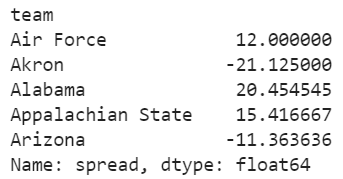
teams['spread'] = np.where(teams['spread'] < -28, -28, teams['spread']) # cap the lower bound scoring margin at -28 pointsIt's now time to calculate the average scoring margin for each team. We'll use the convenient grouping operators in pandas to group the teams data frame by team name.
spreads = teams.groupby('team').spread.mean()
spreads.head()
And here's our output:
Before we get any further, I'd be remiss if I didn't give a shout out to Andrew Mauboussin as a lot of what follows is based on a GitHub repo of his to which someone on Patreon had pointed me. Now that we have the data in the state in which we want it to be, the final steps are to go ahead and perform the SRS calculations. Remember, we will be building a system of 130 equations with 130 unknown variables (so a 130 x 130 matrix). To once again quote Doug Drinen's primer, which was mainly concerned with NFL:
The idea is to define a system of 32 equations in 32 unknowns. The solution to that system will be collection of 32 numbers and those numbers will serve as the ratings of the 32 NFL teams. Define R_ind as Indianapolis' rating, R_pit as Pittsburgh's rankings, and so on. Those are the unknowns. The equations are:
R_ind = 12.0 + (1/16) (R_bal + R_jax + R_cle + . . . . + R_ari)R_pit = 8.2 + (1/16) (R_ten + R_hou + R_nwe + . . . . + R_det)
.
.
.
R_stl = -4.1 + (1/16) (R_sfo + R_ari + R_ten + . . . . + R_dal)
One equation for each team. The number just after the equal sign is that team's average point margin.
Extrapolate this to the 130 teams in FBS. By solving this system of equations, we will find each team's adjusted rating which incorporates scoring margin and strength. I once had a Linear Algebra professor tell me that his course would be the most important undergraduate math course I would ever take. I was dubious then, not so much now.
It's actually not so bad. In order to build up our system of equations, we are going to define two arrays. The first array will define the coefficients for our system of equations and will have dimensions of 130 x 130. The second array will house our solutions and thus be 130 x 1 (one rating for each team). Go ahead and run this code.
# create empty arrays
terms = []
solutions = []

for team in spreads.keys():
    row = []
    # get a list of team opponents
    opps = list(teams[teams['team'] == team]['opponent'])

    for opp in spreads.keys():
        if opp == team:
        	# coefficient for the team should be 1
            row.append(1)
        elif opp in opps:
        	# coefficient for opponents should be 1 over the number of opponents
            row.append(-1.0/len(opps))
        else:
        	# teams not faced get a coefficient of 0
            row.append(0)

    terms.append(row)

    # average game spread on the other side of the equation
    solutions.append(spreads[team])
Okay, we have our system of equations built up, but how do we solve them? Seems like this would be pretty hard, but it's actually the easiest part of this whole guide. The NumPy library contains a linear algebra package which includes a convenient method for solving a system of linear equations. Let's go ahead and solve this system.
solutions = np.linalg.solve(np.array(terms), np.array(solutions))
solutions
It should output the solution to each equation.
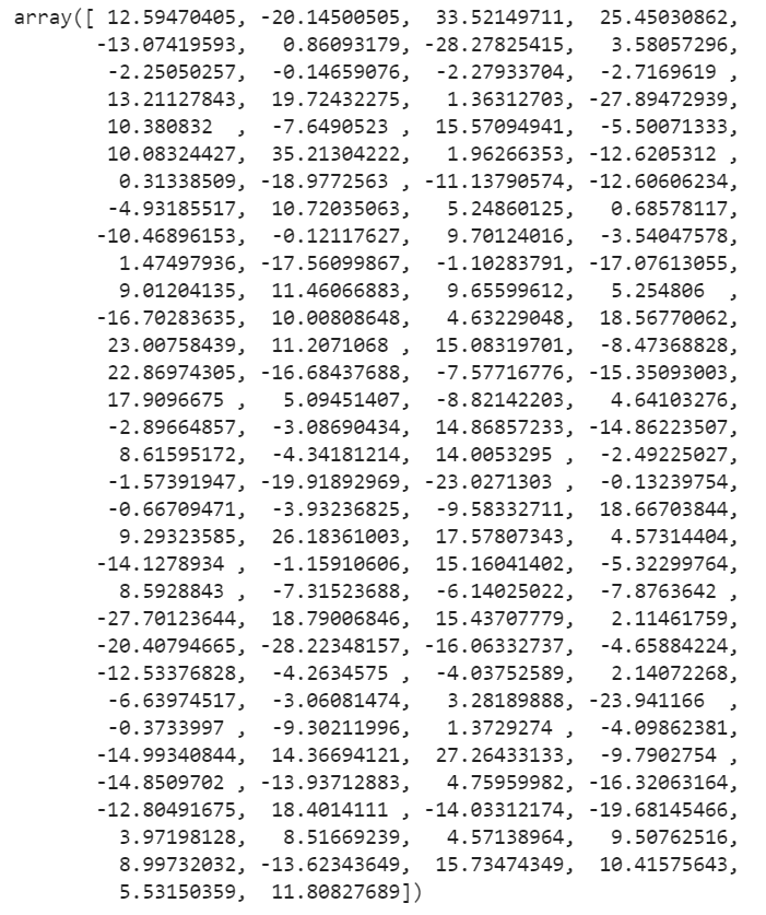
That's not really something we can read as it's all numbers. Let's add team names to this data using Python's zip method. Better yet, let's also create a new pandas DataFrame with this information.
ratings = list(zip( spreads.keys(), solutions ))
srs = pd.DataFrame(ratings, columns=['team', 'rating'])
srs.head()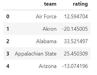
Lastly, there is no ordering here. We have teams matched up with ratings, which is great, but lets order these teams by rating so that we can get some rankings.
rankings = srs.sort_values('rating', ascending=False).reset_index()[['team', 'rating']]
rankings.loc[:24]
And this should output a list of our top 25 teams:
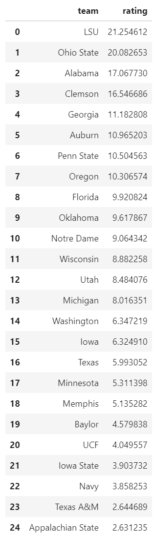
And that's all there is to it. Notice that LSU is ranked #1 at +21.3. This is saying that LSU is 21.3 points better than an average team on a neutral field. Meanwhile, Clemson comes in #4 at +16.5. By these ratings, our SRS model is saying that LSU is a 4.8 point favorite over Clemson on a neutral field (i.e. the National Championship game).
Conclusion
Can this be improved upon? Aboslutely. But, I'll leave that up to you. There are so many ways you can go with this. At a minimum, I recommend at least doing the following:
- Adjust the HFA adjustment
- Remove the HFA adjustment completely
- Mess around with the scoring margin game
- See what happens if you just remove the scoring margin cap
Once you're done tinkering, you can use this as a ratings and ranking system on its own, or you can even incorporate it into a larger system on which you are working. The outputted data makes for an excellent starting point for assessing the strenght of teams and therefore SOS as a whole. But again, that's all up to you.
My Jupyter notebook is now available on GitHub. Feel free to download it and play around. I'm planning on making available any notebooks that result from this series. They will all be included in that same repo under the Talking Tech folder.
Until next time!