
Talking Tech: Predicting Play Calls Using a Random Forest Classifier

Welcome back to Talking Tech! It's been awhile since our last post. To catch everyone up with where we've been thus far, we first went through setting up an environment for data science using Docker and Project Jupyter. When then went over creating a Simple Rating System for college football teams. Most recently, we introduced Plotly and how it can be used to create rich, interactive charts in Python.
In this entry, we're going to dive into machine learning for the first time. As always before we get started, it's important to first have some sort of problem area or something for which we are trying to solve. I've personally done all sorts of models in the past, ranging from predicting game outcomes to ranking and rating teams. One question I haven't really looked at but I think would be interesting to tackle is, would it be possible to predict a coach's play calling based on game situation? Now, it won't be possible to get to a level of granularity where we're breaking down by read options, RPOs, and the like. The data just isn't there yet, at least not with what we have available. However, we certainly can classify things like runs, passes, field goals attempts, and punts.
Random Forests
To achieve this task, we're going to be building a Random Forest Classifier. Random forests are a method of ensemble learning which are quite versatile and relatively easy to set up. The basic gist of ensemble learning is that several different predictive models are created to solve a particular problem. The several different models are then combined into a single model with the goal of producing a final robust model using the power of many.
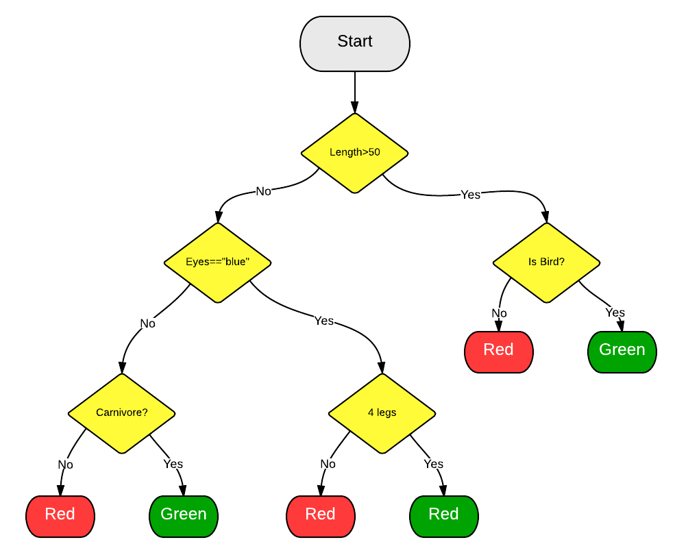
Random forests work by generating tons of decision trees at random. Since these are all generated at random, most won't be that meaningful but to put it simply, all of the "bad" models cancel each other out in the process of making predictions thus allowing the few good trees to surface to the top. So how does that work? Well, when a prediction is made, each decision tree is evaluated based on the inputs. The output of each tree gets tallied and the modal outcome is selected as the final prediction.
A great thing about random forests is that they are super easy to use and are often utilized as an introduction to machine learning. As I mentioned, they are also quite versatile. Not only can they be used to output classifications (i.e. outputting play classifications), but can also be used for regression analysis. We are going to be using the ubiquitous scikit-learn Python library for generating our random forest classifiers. Being more of a newbie to Python myself, I haven't had much exposure to this library until recently, but it's feature set for generating random forests is easy enough to navigate. Maybe we can explore other aspects of this library in future Talking Tech entries. But now let's dig into our play classification model.
Predicting play calls
I don't think there's much value in trying to predict general play call behavior across FBS. In other words, I think it makes most sense to pick a specific coach and try to predict based on their individual play calling behavior. There's too much nuance and variety in offensive style to make building a general model into a futile effort. Mike Leach's play calling patterns are going to differ wildly from Jeff Monken or another service academy coach.
That in mind, we should pick a specific coach to analyze. Being a Michigan fan, I'm going to go with Jim Harbaugh, specifically his tenure at Michigan. Don't care about trying to predict Jim Harbaugh's play calling in different situations? That's totally fine. If you're following along in a Jupyter notebook of your own then feel free to substitute Jim Harbaugh and Michigan with the team and coach of your choice throughout these code snippets.
Retrieving and massaging our data
First thing's first, let's spin up our Jupyter notebook server. If you've been following along, you need only start up your Docker container. The Docker image should have everything we need to get going.
docker run -p 8888:8888 -e JUPYTER_ENABLE_LAB=yes bluescar/jupyterOnce that is loaded up and you've navigated to the Jupyter server in your web browser of choice, go ahead and create a new Python notebook. The first thing we're going to do is to load up some of the standard libraries with which we've been working, namely numpy, pandas, and the Python requests library.
import numpy as np
import pandas as pd
import requests
Now that we're ready to go, it's time to think about what data we need to acquire. The CFBD API should have all the data we need. I'm thinking that the play data makes the most sense for this exercise and it contains all relevant information pertaining to game situation and has convenient labels describing the type of play (run, pass, kickoff, etc). Okay, that's easy enough, but how many years of data should I grab? Jim Harbaugh notably had a four year stint at Stanford prior to jumping from the NFL to Michigan. Do I include that? It's certainly possible that his stint in the NFL had an affect on his play calling behavior, though I don't know. Just to be safe, I'm going to stick with his Michigan tenure, which started in 2015. I recommend doing the same for your coach of choice.
data = pd.DataFrame()
for year in range(2015,2020):
response = requests.get("https://api.collegefootballdata.com/plays?seasonType=both&year={0}&offense=michigan".format(year))
df = pd.io.json.json_normalize(response.json())
data = pd.concat([data, df])
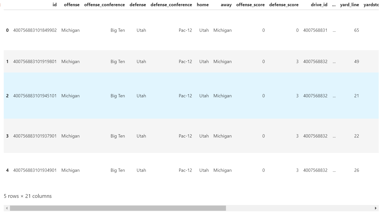
data.head()Like I said, this data was easy enough to grab using the CFBD API's /plays endpoint. I merely had to loop through each of his years at Michigan, starting in 2015. Note that I filtered on plays where Michigan is the offense in my API query. These are the only plays I care about and it is a good API etiquette to grab only the data we need. For one, it's more performant as it greatly reduces the number of plays we need returned to us in each call. It also saves us the step of having to filter the returned data in this manner. Anyway, you should have seen output similar to below for your coach/team of choice.
There's a lot of columns in this data frame that we're not going to need. I don't think things like id fields and play text description are going to help us predict what a play call will be. So let's think about what data is relevant to our endeavor. We obviously want play type as that's going to help us to classify what type of play was called. What things do we think go into how a coach picks what type of play to call? I think we definitely want to look at things like current score, quarter, time remaining, down, distance, and field position. Anything else? Does whether a game is home or away influence play calling? I'm not really sure, so let's add home and away data to find out.
data = data[['home', 'away', 'offense_score', 'defense_score', 'period', 'clock.minutes', 'clock.seconds', 'yardstogoal', 'down', 'distance', 'play_type']]
data.head()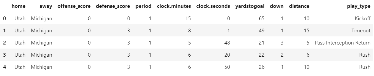
Now this looks much cleaner than what we had before. Is there any more cleanup we need to do? Certainly. We don't necessarily care about which team was home and which was away, but we do care whether the team calling the plays is at home. We can use the home and away labels to create a calculated column called is_home. We'll calculate this field based on whether Michigan is the home team in the play.
data['is_home'] = np.where(data['home'] == 'Michigan', 1, 0)
data.head()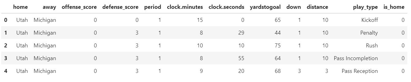
Why did we assign the is_home as o or 1 instead of True/False? In machine learning, you typically need all of your inputs to be in a numerical format. Some libraries may not require this, but instead will convert non-numeric, or categorical, data to be numeric behind the scenes. Data flags, like the is_home distinction, get the same treatment. In most programming languages, specifically those that are not strongly typed, 1 is pretty interchangeable with True and 0 with False.
We still have more things to clean up. How about the clock.minutes and clock.seconds fields? These fields are really all that valuable independent of one another, so let's convert them into a single field which is just the raw seconds remaining.
data['seconds_remaining'] = (data['clock.minutes'] * 60) + data['clock.seconds']
data.head()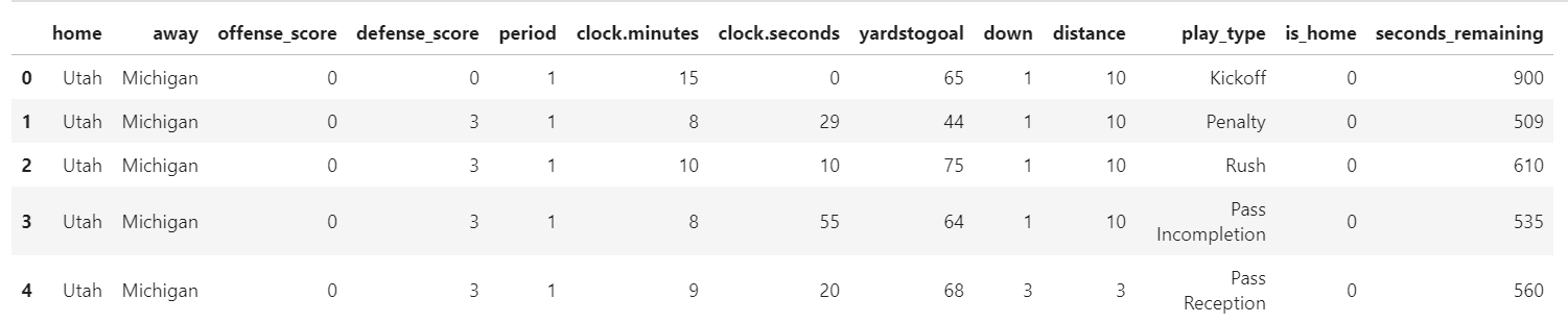
We still have one little bit of cleanup left to go before we can build our random forest classifier. The play_type field is a little too granular for our purposes right now as it currently can describe both what type of play that was called as well as the outcome of the play (e.g. "Pass Incompletion", "Rush TD"). Let's use that column to calculate the outputs we care about. I'm mostly interested in if a rushing or passing play is called. Additionally, I would also like to evaluate a coach's decision to kick punts and field goals. So these will be our four category classifications: rush, pass, punt, FG.
I've gone ahead and written a function to classify play types into one of these four categories. Important to note is that some plays do not fit into any of these classifications. I'm talking things like kick offs, timeouts, and penalties. If a play doesn't fit into any of our four buckets, we're just going to return None for the play call classification. We'll see why in a second. For now, run this snippet of code to define our function and apply it to our data frame to calculate a column for play call.
pass_types = ['Pass Reception', 'Pass Interception Return', 'Pass Incompletion', 'Sack', 'Passing Touchdown', 'Interception Return Touchdown']
rush_types = ['Rush', 'Rushing Touchdown']
punt_types = ['Punt', 'Punt Return Touchdown', 'Blocked Punt', 'Blocked Punt Touchdown']
fg_types = ['Field Goal Good', 'Field Goal Missed', 'Blocked Field Goal']

def getPlayCall(x):
    if x in pass_types:
            return 'pass'
    elif x in rush_types:
        return 'rush'
    elif x in punt_types:
        return 'punt'
    elif x in fg_types:
        return 'fg'
    else:
        return None

data['play_call'] = data['play_type'].apply(getPlayCall)
data.head()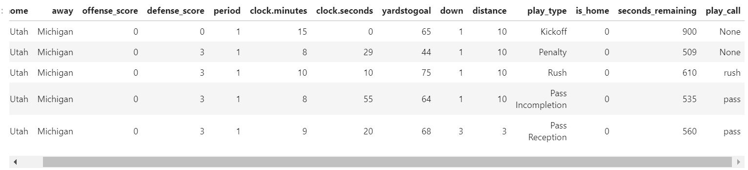
So what about those types plays that don't fit into either of these four play call classifications? We really don't care about these for this exercise. Remember how we set the play call value to None for these rows? Pandas has a very convenient function for straight up dropping rows that have missing values and we can even specify which column or columns we want to be considered when looking for which rows to drop. Run the code below to drop these rows which are outside of our scope.
data.dropna(subset=['play_call'], inplace=True)
data.head()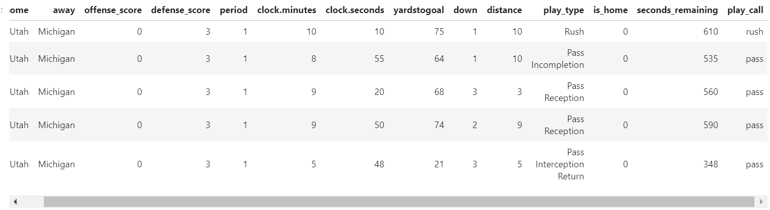
We're almost ready to start building our random forest classifier. Before we do so, let's get rid of any remaining columns that are no longer needed, namely those columns which we used purely for calculating new columns. I'm going to store this data frame into a new variable so that these columns are still available should we want to go back and do any further tweaking.
plays = data[['offense_score', 'defense_score', 'period', 'yardstogoal', 'down', 'distance', 'is_home', 'seconds_remaining', 'play_call']]
plays.head()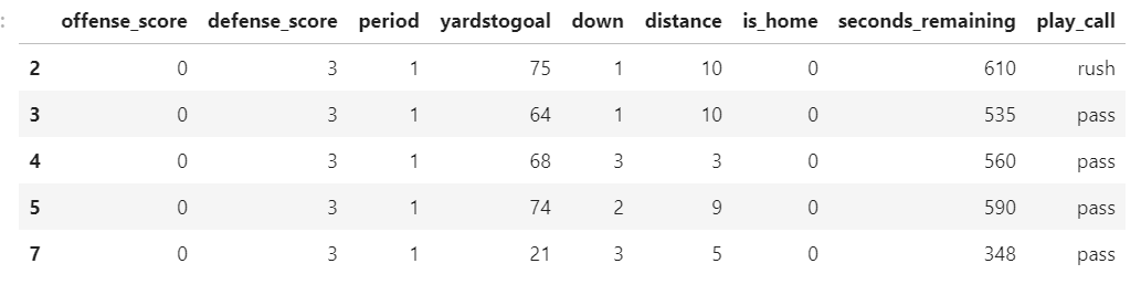
Now we're ready to get building!
Building a prediction model
As I mentioned earlier, we'll be using the versatile scikit-learn library to build our model. If you're using the Docker image, this library is already builtin. If not, you'll need to go install it. We're going to go ahead and import two modules from the library which we'll be using. The first module provides convenient functionality for splitting data into training and validation sets. We'll talk about that more in a sec. The second module is the main module used for building random forest classifiers.
from sklearn.model_selection import train_test_split
from sklearn.ensemble import RandomForestClassifier
Now we're going to split up a data a little bit to make it more conducive towards building our model. The first thing we are going to do is separate our set of features (our independent variables) from what we want our model to output (our dependent variable). We want our model to be able to take in a set of inputs regarding the game situation and use those inputs to predict play calls. Our dependent variable is the set of play calls, so everything else belongs in our feature set. The second thing we are going to do is to split our data into training and validation sets. Using the convenient train_test_split module we imported above, we are going to pull out 20% of the data to use as a validation set.
# split the data set between our independent variables (i.e. features) and our dependent variable or output
play_calls = plays['play_call']
plays = plays.drop(['play_call'], axis=1)

# split the data into training and validation sets
plays_train, plays_validation, calls_train, calls_validation = train_test_split(plays, play_calls, train_size=0.8, test_size=0.2, random_state=0)
plays_train.head()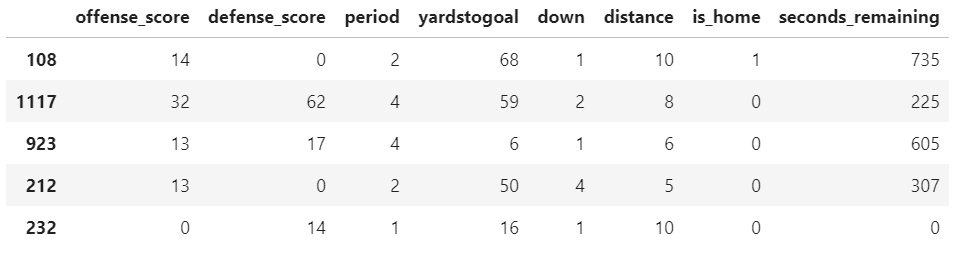
Why have a separate validation set? One danger in machine learning is the potential threat of overfitting. We know our model will be accurate when outputting predictions on our training set. I mean, that makes sense. It should be accurate and predicting that very data that was used to train it, but what good is that? I should be able to apply any model I train to any other potential set of inputs and get accurate results. Overfitting occurs when your model learns from the training set a little too good such that it's predictions are only good on the set on which it was trained. Think of it as analogous to the model basically memorizing your training set and as a result, it simply does not perform well on outside data. We split out a validation set so that we can test out our model and ensure it is accurately predicting for the problem we are trying to solve.
Remember earlier when I mentioned that you generally want all of your data in a numerical format for training? Is all of our data currently in a numerical format? Our feature set certainly is, but our dependent set of play calls are not. But how do we convert categorical data into numbers? This is simple enough to do with pandas, largely because we have a very simple set that contains only four distinct categories (pass, rush, punt, fg). scikit-learn has some features for handling more complex scenarios, but that's outside the scope of this post. Run the following code to convert our outputs into numerical format.
y, y_keys = pd.factorize(calls_train)We used the factorize method in pandas to convert our output data into numeric format. It returned two sets to us, one contained the data as a set of numbers ranging from 0 to 3 and other containing the key mappings telling us which number mapped to which label. We are now ready to train our model. Run the following code to build and train a random forest classifier.
# build the classifier
classifier = RandomForestClassifier(random_state=0, n_estimators=100)

# train the classifier with our test set
classifier.fit(plays_train, y)
Note that we passed in both our set of features (plays_train) as well as our set of corresponding outputs in numeric format (y). Now, let's pass in our validation set of features and see what the classifier outputs.
classifier.predict(plays_validation)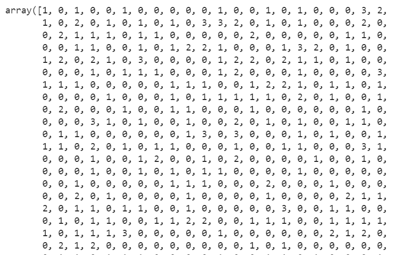
Not very useful output, is it? That's because we are looking at the raw outputs and still need to convert them into labels using the y_keys mapping object we created earlier. Before we do that, I want to show you one cool feature provided to us in the scikit-learn library. Run this snippet.
classifier.predict_proba(plays_validation)[0:10]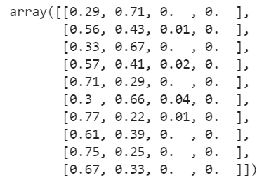
What's going on here? In contrast to the regular predict method which just outputs a single predicted value for each set of inputs, the predict_proba provides a greater level of granularity by outputting the probabilities for each set of inputs. Notice that we have four probabilities for each set of inputs which correspond to our four different output labels (pass/rush/fg/punt). We won't go any further with this specific area of functionality, but it's certainly interesting to note.
Now let's get back to mapping our original set of outputs to our category labels. It's actually pretty simple. Just run the following line of code.
predicted_calls = y_keys[classifier.predict(plays_validation)]
predicted_calls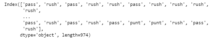
Again, not the most useful output but we're making some progress. What would be really valuable is if we could somehow compare the predicted outputs with the actual outputs from our validation set. We can use the crontab functionality in pandas to do just that.
pd.crosstab(calls_validation, predicted_calls, rownames=['Actual Calls'], colnames=['Predicted Calls'])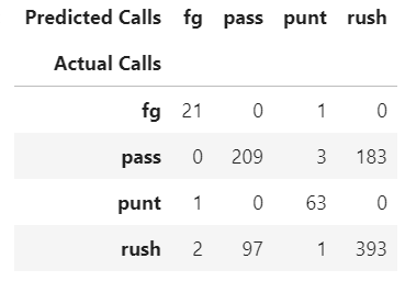
What is this telling us here? Each row represents the actual classification of play calls in our validation set. The columns represent what our classifier predicted the play calls to be. As you can see, it's pretty accurate in predicting when Jim Harbaugh punts and when he kicks field goals. It's also doing pretty decent on predicting called run plays, but not so much on passing plays. There's definitely room for improvement.
aImproving our model
Let's evaluate how our model is making predictions to see where we can improve. Using the builtin feature_importances_ property, we can actually see how it is weighting the importance of each feature in making its predictions.
list(zip(plays_train, classifier.feature_importances_))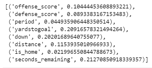
As you can see, it's placing the most weight on seconds remaining in the quarter, down, and yards to the goal line. It's not really doing much with our home/away flag. Since there's a possibility that it's just adding noise at this point, let's go ahead and get rid of that column and see what happens. Are there any other changes we can make? It's not doing much with the period field, let's wrap that into seconds remaining, much like we did with minutes earlier.
# incorporate period into seconds_remaining
plays['seconds_remaining'] = ((4 - plays['period']) * 15 * 60 ) + plays['seconds_remaining']

# drop is_home and period columns
plays = plays.drop(columns=['is_home', 'period'])
From here, we're pretty much going to copy and paste our earlier code snippets and consolidate them. Let's see if anything improved.
plays_train, plays_validation, calls_train, calls_validation = train_test_split(plays, play_calls, train_size=0.8, test_size=0.2, random_state=0)
y, y_keys = pd.factorize(calls_train)

classifier = RandomForestClassifier(n_estimators=100, random_state=0)
classifier.fit(plays_train, y)

predicted_calls = y_keys[classifier.predict(plays_validation)]

pd.crosstab(calls_validation, predicted_calls, rownames=['Actual Calls'], colnames=['Predicted Calls'])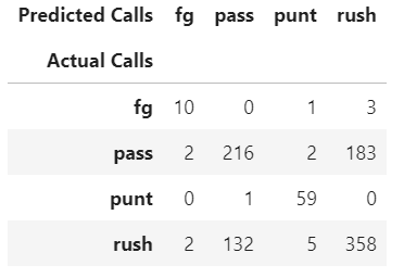
Did that improve things at all? Not really. Our accuracy in predicting rushing play calls got worse. Everything else either stayed the same or improved only marginally. Let's look at how the feature weights changed.
list(zip(plays_train, classifier.feature_importances_))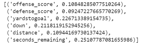
Look at our offense_score and defense_score fields. Do we really need both of them? It seems like play calling would be more a function of how much a team is behind or ahead rather than the raw scores. What happens if we convert them into a single field for score margin? Let's find out.
# calculate new scoring margin field and drop the individual score columns
plays['margin'] = plays['offense_score'] - plays['defense_score']
plays = plays.drop(columns=['offense_score', 'defense_score'])

plays_train, plays_validation, calls_train, calls_validation = train_test_split(plays, play_calls, train_size=0.8, test_size=0.2, random_state=0)
y, y_keys = pd.factorize(calls_train)

classifier = RandomForestClassifier(n_estimators=100, random_state=0)
classifier.fit(plays_train, y)

predicted_calls = y_keys[classifier.predict(plays_validation)]

pd.crosstab(calls_validation, predicted_calls, rownames=['Actual Calls'], colnames=['Predicted Calls'])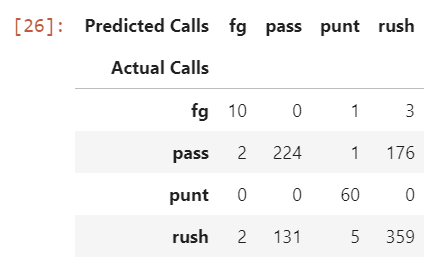
Predictions of passing plays improved. Rushing play call predictions mostly stayed the same from our last model. At this point, we are perfectly predicting punt calls and are pretty close to perfect with field goal calls.
There's certainly more things we can do to improve the model, but let's look at how we can use the model to evaluate real-time data. I'm going to define a function that takes in inputs for yard line, down, distance, seconds remaining, and score margin.
def predict_call(yards, down, distance, seconds, margin):
    test_plays = pd.DataFrame({'yardstogoal': [yards], 'down': [down], 'distance': [distance], 'seconds_remaining': [seconds], 'margin': [margin]})
    return y_keys[classifier.predict(test_plays)][0]
Let's say the ball is at the 50 yard line. It's 4th and 1 with 3 minutes left and Michigan is down by 4 points. What does Michigan do?
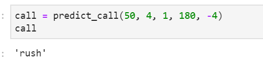
Our model predicts that Jim Harbaugh will go for it by calling a run play. Now let's say that Michigan is in the exact same scenario, but up by 10 points instead of down by 4. Does the call change?
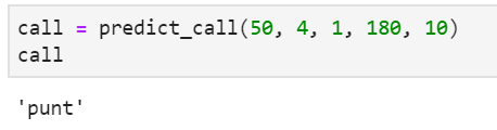
The model thinks that Jim Harbaugh will decide to punt here. I think both of these outputs are pretty reasonable for someone who has watched a lot of Michigan football. It's always important to ensure your model at least passes the eyeball test and we're there for these two scenarios.
What now?
Well, I'm not quite sure we would call this model "production-ready" to the point where we're actually able to start disseminating results from it. There's a lot more work we can do here, but I'll leave that to you. Our main purpose with this series to just to go over what tools are available and demonstrate potential use cases. The rest is always up to you.
And perhaps your results are more accurate than mine if you used a different coach. Note how accurate we are in calling punt and FG situations compared to runs and passes. Why might that be? For one, these are the types of decisions that are pretty solidly the domain of a head coach. There's also much less nuance. A punt is a punt and a FG attempt is a FG attempt. Other plays are more nuanced. We're not really classifying things like RPOs or QB scrambles and so those things can throw our pass/run numbers off.
Another thing to note is that the head coach may not even be the one calling pass vs run, whereas they most certainly are the ones making punt and FG determinations. So it might make more sense to do this exercise by OC rather than HC. Jim Harbaugh is traditionally known to call his own offense, however he notoriously ceded control of his offense this past season to newcomer Josh Gattis. It might make more sense to look at years Harbaugh was calling plays separately from the year in which Gattis was calling them.
There certainly are other things we can tweak. One thing related to the above might be sample size. Five season may just be too much data. It's certainly possible that a player caller evolves with the game or depending on the staff he is surrounded with. It might make more sense to train on a single season or two's worth of data at a time.
There are many different angles you can take this. Some exercises I recommend:
- Isolate your data by offensive coordinator rather than by head coach. Does this improve things?
- Are there any data points you can add or modify to give a more accurate model?
- Remember the snippet where we broke the prediction into a list of probabilities for each outcome? Is there anything we can do with that.
- Lastly, are there any other CFB-related applications for which a random forest classifier may be a good option? Try it out.
We may continue exploring random forests in further entries in the series. We're definitely going to keep diving into machine learning. Eventually, we'll be looking into building our own neural networks, which is an area in which I've had a lot of experience. Stay tuned!
Further Learning
- Check out the Jupyter notebook from this post on GitHub
- Random Forests in Python by The Yhat Blog
- scikit-learn documentation
- Kaggle's Intro to Machine Learning micro-course